Thinking and Reasoning

An Introduction to the Psychology of Reason, Judgment and Decision Making

Ken Manktelow, Niall Galbraith

• Publisher: Psychology Press
• Year: 2012
• eBook ISBN: 9781136295232
• Topic: Psychology
• Subtopic: Cognitive Psychology & Cognition
• Index: Psychology

The area of psychological research reviewed in this book is one that is not only increasing in popularity in college curricula, but is also making an ever larger impact on the world outside the classroom. Drawing upon research originally cited in Ken Manktelow's highly successful publication Reasoning and Thinking, this completely rewritten textbook reflects on the revolutionary changes that have occurred in the field in recent years, stemming from the huge expansion in research output, as well as new methods and explanations, and the appearance of numerous books on the subject aimed at the popular market.

The main areas covered are probability judgment, deductive and inductive reasoning, decision making, hypothetical thinking and rationality. In each case, the material is almost entirely new, with topics such as the new paradigm in reasoning research, causal reasoning and counterfactual thinking appearing for the first time. The book also presents an extended treatment of decision making research, and contains a chapter on individual and cultural influences on thinking.

Thinking and Reasoning provides a detailed, integrated and approachable treatment of this area of cognitive psychology, and is ideal reading for intermediate and advanced undergraduate students; indeed, for anyone interested in how we draw conclusions and make choices.

Chapter 1

Judging and thinking about probability

Defining probability

Judging plain probabilities

Belief updating

Summary

If you have read the Preface, you will have been cued into the importance of probability in how we now understand and explain thinking and reasoning. We therefore open with this central topic: it forms the basis of explanation across the spectrum of thought. In this chapter, we shall look at research that assesses how people judge probability directly. You may have come across the word in statistics classes, and already be stifling a yawn. If so, wake up: probability is far from being just a dry technical matter best left in the classroom. Everyone judges probability, and does so countless times every day. You might have wondered today whether it is going to rain, how likely you are to fall victim to the latest flu u outbreak, whether your friend will be in her usual place at lunchtime, and so on.

How do we make these judgments? We can make a comparison between normative systems, which tell us what we ought to think, and descriptive data on how people actually do think. To get you going in doing this, here are some questions devised by my statistical alter ego, Dr Horatio Scale. Answering them will raise the probability that you will appreciate the material in the rest of this chapter. We shall look at the answers in the next section.

1 a What is the probability of drawing the ace of spades from a fair deck of cards?

b What is the probability of drawing an ace of any suit?

c What is the probability of drawing an ace or a king?

d What is the probability of drawing an ace and then a king?

2 You are about to roll two dice. What is the chance that you will get ‘snake eyes’ (double 1)?

3 a What is the chance that you will win the jackpot in the National Lottery this week?

b What is the chance that you will win any prize at all this week?

(The British lottery lets you choose six numbers from 1 to 49. You win the jackpot if all your six numbers are drawn; you win lesser prizes if three, four or five of your numbers are drawn.)

4 Yesterday, the weather forecaster said that there was a 30% chance of rain today, and today it rained. Was she right or wrong?

5 What is the chance that a live specimen of the Loch Ness Monster will be found?

6 Who is more likely to be the victim of a street robbery, a young man or an old lady?

7 Think about the area where you live. Are there more dogs or cats in the neighbourhood?

Defining probability

The phrase ‘normative systems’, plural, was used above because even at the formal level, probability means different things to different people. It is one of the puzzles of history that formal theories of probability were only developed comparatively recently, since the mid-17th century. Their original motivations were quite practical, due to the need to have accurate ways of calculating the odds in gambling, investment and insurance. This early history is recounted by Gigerenzer, Swijtink, Porter, Daston, Beatty and Krüger (1989) and by Gillies (2000). Gillies solves the historical puzzle by pointing to the use of primitive technology by the ancient Greeks when gambling, such as bones instead of accurately machined dice, and to their lack of efficient mathematical symbol systems for making the necessary calculations – think of trying to work out odds using Roman numerals. All four of the formal definitions of probability that are still referred to have been developed since the early 20th century. Here they are.

Logical possibility

Probability as logical possibility really only applies to objectively unbiased situations such as true games of chance, where there is a set of equally probable alternatives. We have to assume that this is the case when working out the odds, but it is hard to maintain this stipulation in real life. This is behind Gillies’ explanation of why the ancient Greeks and Romans could not develop a theory of probability from their own games of ‘dice’ made from animal bones: these have uneven sides that are consequently not equally likely to turn up.

To see how we can work out odds using logical possibility, let us take Dr Scale’s first question, and assume that we are dealing with a properly shuffled, fair deck of cards, so that when we draw one from it, its chances are the same as any other’s. There are 52 cards in the deck, only one of which is the ace of spades, so its odds are 1:52. Odds are often expressed in percentages: in this case, it is about 1.92%. Probability in mathematics and statistics is usually given as a decimal number in the range between 0 and 1: in this case, it is .0192. An ace of any suit? There are four of them, so we can work out 4:52 (i.e. 1:13) in the same way, or multiply .0192 by four to obtain the answer: .077.

The odds of an ace or a king are the odds of each added together: there is one of each in each suit of 13 cards, so the joint odds are 2:13, or .154. Question 1d is a bit more complicated. It introduces us to the idea of conditional probability, because we need to calculate the probability of a king given that you have drawn an ace. Each has the probability .077, and you obtain the conditional probability by multiplying them together, which gives the result of just under .006, i.e. 6:1000 – a very slim chance.

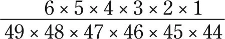
Now you can address Dr Scale’s third question, the lottery odds. With 49 numbers to choose from, the odds of the first are clearly 1:49. This number is no longer available when you come to choose the second number, so its odds are 1:48, and so on. Sticking with just these two for a moment, the odds of your first one and then your second one coming up can be worked out just as with the ace and king: 1:49 × 1:48, or .0204 × .0208 = just over .0004. But with the lottery, the order in which the numbers are drawn does not matter, so we have to multiply that number by the number of orders in which these two numbers could be drawn. That is given by the factorial of the number of cases, in this case 2 × 1 = 2. This number replaces the 1 in the odds ratio, which now becomes 2:49 × 48. You simply expand this procedure to work out the chances of 6 numbers out of 49 being drawn in any order. If you want to do this yourself, it is probably easiest to use the numbers in the following form and then use cancelling, otherwise the long strings of zeroes that will result if you use the decimal notation will boggle your calculator:

The top line is factorial 6, for the number of orders in which six numbers could appear. The resulting odds are approximately 1:13.98 million. So if you play once a week, you can expect to win the jackpot about once every quarter of a million years.

Question 3b asked about the odds of winning any prize at all. You can work out the odds of three, four or five of your numbers coming up in exactly the same way as just described. You don’t just add all these results together, however, because there are numerous ways in which, say, three numbers from the six you have chosen can come up. So you have to multiply each odds result by this number, and then add them all up. In case you don’t feel up to it, I can tell you that the odds of winning any prize in any one week are around 1:57. So a regular player should get a prize about once a year, although this will almost certainly be the lowest prize (the odds of three of your numbers coming up are about 1:54). I shall deal with whether, in the face of these odds, playing the lottery is a good decision in Chapter 8.

Frequency

Frequency theory has roots that go back to the 19th century, but it was developed in most detail in the mid-20th, and has been highly influential ever since. In psychology, this influence has been even more recent, as we shall see later in this chapter. People who adopt frequency theory are called frequentists, and they regard probability as the proportion of times an event occurs out of all the occasions it could have occurred, known as the collective. There are two kinds of collectives, referred to by an early frequentist, von Mises (1950), as mass phenomena or repetitive events.

Dr Scale’s sixth question can be taken as a frequency question about a mass phenomenon: you could count up the number of street robberies and look at the proportions where the victims were old ladies and young men, and see which was the greater. Games of chance, such as coin flips, dice and lotteries, can also be analysed in terms of frequencies: these are repetitive events. Instead of working out the odds mathematically, you could count up the number of jackpot winners as the proportion of players, for instance. Over time, the results of the two probabilities, frequency and odds, should converge; if they don’t, you have detected a bias. Gamblers can be exquisitely sensitive to these biases: Gillies (2000) tells us about a 17th century nobleman whose was able, through his extensive experience with dice games, to detect the difference between odds of .5000 and .4914, a difference of 1.7%. Question 7 (cats and dogs) is also a frequency question, again about a mass phenomenon. Beware: this question has a catch, which we shall return to later in the chapter.

Propensity

For a true frequentist, it makes no sense to ask for the probability of a single event such as how likely you are to win a game of chance, because the only objective probabilities are frequencies – things that have actually happened – and frequencies cannot be derived from one-off observations or events that have not yet occurred. Nor can frequencies have any ‘power’ to influence a single observation: suppose there are twice as many dogs as cats in your area, does that fact determine in any way the species of the next pet you see? How could it? But everyone has a strong feeling that we can give such odds: we do feel that the next animal is more likely to be a dog than a cat. This clash of intuitions was addressed by the celebrated philosopher of science, Karl Popper (1959a), who introduced the propensity theory. He needed to do so because of single events in physics, such as those predicted by quantum mechanics. The probabilities of such events must, he thought, be objective, but they could not be based on frequencies.

Dr Scale’s second question is about propensity: note that it asks you specifically about a single event, the next throw, whereas Question 1 was more general. Popper used a dice game example when he tried to solve the intuitive riddle just described (i.e. an example involving logical possibility). Consider two dice, one fair and one weighted so that it is biased in favour of showing a 6 when tossed: it tends to show a 6 on one-third of the throws (i.e. twice as often as it would if unbiased). Suppose we have a long sequence of dice throws, most involving the biased die with occasional throws of the fair one. Take one of these fair tosses. What is the probability that it will show a 6? Popper argued that a frequentist would have to say 1:3, because the ‘collective’ set of throws has produced this frequency. However, you and I know that it must be 1:6, because we are talking about the fair die, and fair dice will tend to show each of their six sides with the same frequency.

Popper’s solution was to appeal to the difference in causal mechanisms embodied in the two dice to resolve this paradox: the collective really consists of two sub-collectives that have been produced by two different generating conditions. The biased die has the propensity to show a 6 more often than a fair die does because of its different causal properties. (We shall look in detail at causal thinking in Chapter 4.)

There are problems with propensity theories (others have come after Popper), one of which is that invoking causal conditions just replaces one set of problems with another. In the real world, it can be very difficult to produce the same generating conditions on different occasions, as all psychology students know from the discussion of confounding variables in their methodology courses. If it is not realistically possible to repeat these conditions, then is an objective single-event probability therefore also not possible? And if so, what is the alternative?

Degree of belief

We have strong intuitions about the probability of single events, so the alternative to objective probabilities must be subjective probabilities, or degrees of belief. Look at Dr Scale’s fifth question. If you have heard of the Loch Ness Monster, you will have some view as to how likely it is that it really exists. However, this cannot be based on a logical possibility, nor can it be based on a frequency: there is not a ‘mass’ of equivalent Scottish lochs, some with monsters and some without. Perhaps you can even assign a number to your belief, and perhaps you use objective facts in doing so, to do with the known biology and ecology of the species that you presume the beast to be. But your degree of belief can only be subjective.

Now look at Dr Scale’s fourth question, about the weather forecast. Weather presenters often use numbers in this way, but what do they mean? Once again, it is hard to see how this can be a logical possibility: weather is not a series of random, equivalent events, even in Britain. Could it then be a frequency? If so, what of? This particular date in history, or days when there has been a weather pattern like this? Baron (2008) uses weather forecasts as an example by which we can assess how well someone’s probabilistic beliefs are calibrated. That is, if someone says that there is a 30% chance of rain, and it rains on 30% of days when she says this, then her judgment is well calibrated (this is another kind of frequency). This may be useful information about the climate, but it is not a useful attitude to weather forecasting: we want to know whether to cancel today’s picnic, a single event. And if the forecaster said 30%, and it rained today, isn’t she more wrong than right? She implied that there was a 70% chance that it would not rain. Thus you can be well calibrated in frequency terms but hopeless at predicting single events.

Confusion over the use of percentages like this was addressed by Gigerenzer, Hertwig, van den Broek, Fasolo and Katsikopoulos (2005), following up an earlier study by Murphy, Lichtenstein, Fischhoff and Winkler (1980). First of all, they set the normative meaning of this figure: that there will be rain on 30% of days where this forecast figure is given. So they are adopting the frequentist approach. They tested people’s understanding of the figure in five different countries, varying according to how long percentage forecasts had been broadcast. The range was from almost 40 years (New York, USA: they were introduced there in 1965) to never (Athens, Greece). The prediction was that the degree of ‘normative’ understanding would be correlated with length of usage of percentage forecasts. It was. Alternative interpretations produced by participants were that the 30% figure meant that it would rain for 30% of the time, or across 30% of the region. Note, by the way, that even among the New Yorkers about one-third did not give the ‘days’ interpretation. And keep in mind that people listen to weather forecasts to find out about particular days, not climatic patterns. Gigerenzer et al. urge that forecasters be clear about the reference class when giving numerical probabilities. This is an important issue that we shall return to in a short while.

By the way, my degree of belief in the Loch Ness Monster is close to zero. If, as most of its publicity says, it is a plesiosaur (a large aquatic reptile of a kind that existed at the end of the Cretaceous period, 65 million years ago), we would have to have a breeding population. They were air breathers – heads would be bobbing up all over the place. They would not be hard to spot.

Of course, our beliefs in rain or monsters can be changed if we encounter some new evidence. You go to bed with a subjective degree of belief in rain tomorrow at .3, and wake up to black skies and the rumble of thunder: that will cause you to revise it.

Belief revision: Bayes’ rule

The subjective view of probability opens up a range of theoretical possibilities, which all come under the heading of the Bayesian approach to cognition. It is hard to overestimate the influence of this perspective at the present time (see Chater & Oaksford, 2008, for a recent survey), and we shall see it applied to theories of reasoning in later chapters....

Table of contents

• Cover
• Halftitle
• Title
• Copyright
• Contents
• Dedication
• Preface
• 1. Judging and thinking about probability
• 2. The study of reasoning: classic research
• 3. Reasoning with propositions
• 4. Reasoning and meaning
• 5. Explaining reasoning: the classic approaches
• 6. Explaining reasoning: the ‘new paradigm’
• 7. Hypothetical thinking: induction and testing
• 8. Decision making: preference and prospects
• 9. Decisions in context
• 10. Thinking, reasoning and you
• Notes
• References
• Author index
• Subject index