Mathematics for Biological Scientists

Mike Aitken, Bill Broadhurst, Stephen Hladky

• Publisher: Garland Science
• Year: 2009
• Print ISBN: 9780815341369
• eBook ISBN: 9781136843921
• Edition: 1
• Topic: Biological Sciences
• Subtopic: Biology
• Index: Biological Sciences

Mathematics for Biological Scientists is a new undergraduate textbook which covers the mathematics necessary for biology students to understand, interpret and discuss biological questions.

The book's twelve chapters are organized into four themes. The first theme covers the basic concepts of mathematics in biology, discussing the mathematics used in biological quantities, processes and structures. The second theme, calculus, extends the language of mathematics to describe change. The third theme is probability and statistics, where the uncertainty and variation encountered in real biological data is described. The fourth theme is explored briefly in the final chapter of the book, which is to show how the 'tools' developed in the first few chapters are used within biology to develop models of biological processes.

Mathematics for Biological Scientists fully integrates mathematics and biology with the use of colour illustrations and photographs to provide an engaging and informative approach to the subject of mathematics and statistics within biological science.

CHAPTER 1

Quantities and Units

Figure 1.1
The authors, Mike, Steve, and Bill, holding a protein sample destined for the 500 MHz NMR spectrometer in the background. Image courtesy of Mike Aitken, Bill Broadhurst, and Steve Hladky.

As scientists, we need to make quantitative statements about the physical quantities measured in our experiments. Algebra provides the language and grammar to make these statements. In this language the sentences are equations or inequalities whereas the words are symbols. A symbol may stand for a physical quantity or a number; for an operation such as addition or multiplication; or for a relationship such as ‘is equal to’ or ‘is greater than’. Often we use letters such as x, t, m, or A to stand for physical quantities such as distance, time, mass, or area. Symbols can also be special characters such as + for addition, or a combination of letters such as ‘sin’ for the sine function introduced in Chapter 4.

A physical quantity is a combination of a numerical value and a unit, for example a length of 1 m, a time of 2 s, or a mass of 70 kg, where the ‘m’ stands for meter, ‘s’ for second, and ‘kg’ for kilogram. Both are needed; if we change the unit the number changes accordingly. Many of the laws of science are expressed as simple equations relating physical quantities. A familiar example is F = ma where F, m, and a stand for force, mass, and acceleration. There are various systems for choosing units and conventions for how physical quantities are to be described. In this book we use the Système Internationale (SI) system of units, which has become standard for scientists and engineers throughout the world.

1.1 Symbols, operations, relations, and the basic language of mathematics

In the language of mathematics, the words are symbols like x, t, m, +, ×, ÷, =, >. Symbols can stand for numbers or for physical quantities; they can indicate operations or they can state relationships like ‘is equal to’ or ‘is greater than’. You first started using many of these symbols back in primary school where you learned what + and = mean. Even then you also used symbols to stand for unknown numbers in exercises like that shown in Figure 1.2.

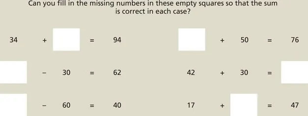
Figure 1.2
In elementary arithmetic, we may have thought of ☐ as just a space holder to tell us where to write the answer, but it can also be regarded as a symbol that stands for a number whose value is not already known.

You may have thought of ☐ as just a box to tell you where to write the answer, but it can also be regarded as a symbol called ‘box’ that stands for a number whose value is not already known. The equation ☐ + 3 = 8 tells us a relation between ☐ and the numbers 3 and 8, and this relation allows us to solve for the value, 5, to be assigned to the variable ‘box’. That really is the crux of using algebra; it allows us to state relations before we know the actual values. Of course the relations between our symbols are going to be a bit more complicated – but the principle behind the use of algebra is still the same.

Note that whenever algebraic expressions are typeset, the letters used in a symbol are written in italics if the symbol represents either a number or a physical quantity. By contrast plain roman type is used for symbols that represent units or labels. Typographical conventions like these are fiddly but they can be very important. For example, in the equation for the gravitational force on an object at the earth’s surface,

$F=mg=m\times 9.8\text{m}{\text{s}}^{-2},$

(EQ1.1)

m and m are completely different. The italic type tells us that m stands for a physical quantity, mass, which might be expressed in kilograms; the plain roman type for the m after the 9.8 tells us it stands for the unit, meter.

Symbols and algebra can be used to express very profound notions. For instance E can represent the total energy of a chunk of matter, m its mass, and c the speed of light. Combining these with the symbol for ‘is equal to’ and the notation for raising to a power Einstein wrote

$E=m{c}^2.$

(EQ1.2)

That bit of shorthand is a lot more compact and a lot more famous than its equivalent in English, ‘The total energy of an object is equal to its mass multiplied by the square of the speed of light.’ However, and this is the important point for now, the algebra and the English are being used to say exactly the same thing.

Now consider a very simp...

Table of contents

• Cover
• Half Title
• Title Page
• Copyright Page
• Table of Contents
• Preface
• Introduction
• Chapter 1 Quantities and Units
• Chapter 2 Numbers and Equations
• Chapter 3 Tables, Graphs, and Functions
• Chapter 4 Shapes, Waves, and Trigonometry
• Chapter 5 Differentiation
• Chapter 6 Integration
• Chapter 7 Calculus: Expanding the Toolkit
• Chapter 8 The Calculus of Growth and Decay Processes
• Chapter 9 Descriptive Statistics and Data Display
• Chapter 10 Probability
• Chapter 11 Statistical Inference
• Chapter 12 Biological Modeling
• Answers to End of Chapter Questions
• Appendices
• Index