Multiple Regression and Beyond

An Introduction to Multiple Regression and Structural Equation Modeling

Timothy Z. Keith

• Publisher: Routledge
• Year: 2019
• ISBN:
  9781351667920
• Edition: 3
• Topic: Education
• Subtopic: Research in Education

Companion Website materials: https://tzkeith.com/

Multiple Regression and Beyond offers a conceptually-oriented introduction to multiple regression (MR) analysis and structural equation modeling (SEM), along with analyses that flow naturally from those methods. By focusing on the concepts and purposes of MR and related methods, rather than the derivation and calculation of formulae, this book introduces material to students more clearly, and in a less threatening way. In addition to illuminating content necessary for coursework, the accessibility of this approach means students are more likely to be able to conduct research using MR or SEM--and more likely to use the methods wisely.

This book:
• Covers both MR and SEM, while explaining their relevance to one another
• Includes path analysis, confirmatory factor analysis, and latent growth modeling
• Makes extensive use of real-world research examples in the chapters and in the end-of-chapter exercises
• Extensive use of figures and tables providing examples and illustrating key concepts and techniques

New to this edition:
• New chapter on mediation, moderation, and common cause
• New chapter on the analysis of interactions with latent variables and multilevel SEM
• Expanded coverage of advanced SEM techniques in chapters 18 through 22
• International case studies and examples
• Updated instructor and student online resources

Part I
Multiple Regression

1
Simple Bivariate Regression

Simple Bivariate Regression

Example: Homework and Math Achievement

Regression in Perspective

Relation of Regression to Other Statistical Methods

Explaining Variance

Advantages of Multiple Regression

Other Issues

Prediction Versus Explanation

Causality

Review of Some Basics

Variance and Standard Deviation

Correlation and Covariance

Working With Extant Data Sets

Summary

Exercises

Notes

This book is designed to provide a conceptually-oriented introduction to multiple regression along with more complex methods that flow naturally from multiple regression: path analysis, confirmatory factor analysis, and structural equation modeling. In this introductory chapter, we begin with a discussion and example of simple, or bivariate, regression. For many readers, this will be a review, but, even then, the example and computer output should provide a transition to subsequent chapters and to multiple regression. The chapter also reviews several other related concepts, and introduces several issues (prediction and explanation, causality) that we will return to repeatedly in this book. Finally, the chapter relates regression to other approaches with which you may be more familiar, such as analysis of variance (ANOVA). I will demonstrate that ANOVA and regression are fundamentally the same process and that, in fact, regression subsumes ANOVA.

As I suggested in the Preface, we start this journey by jumping right into an example and explaining it as we go. In this introduction, I have assumed that you are familiar with the topics of correlation and statistical significance testing and that you have some familiarity with statistical procedures such as the t test for comparing means and analysis of variance. If these concepts are not familiar to you a quick review is provided in Appendix B. This appendix reviews basic statistics, distributions, standard errors and confidence intervals, correlations, t tests, and ANOVA.

Simple Bivariate Regression

Let’s start our adventure into the wonderful world of multiple regression with a review of simple, or bivariate, regression; that is, regression with only one influence (independent variable) and one outcome (dependent variable).¹ Pretend that you are the parent of an adolescent. As a parent, you are interested in the influences on adolescents’ school performance: what’s important and what’s not? Homework is of particular interest because you see your daughter Lisa struggle with it nightly and hear her complain about it daily. A quick search of the Internet reveals conflicting evidence. You may find books (Kohn, 2006) and articles (Wallis, 2006) critical of homework and homework policies. On the other hand, you may find links to research suggesting homework improves learning and achievement (Cooper, Robinson, & Patall, 2006). So you wonder if homework is just busywork or is it a worthwhile learning experience?

Example: Homework and Math Achievement

The Data

Fortunately for you, your good friend is an 8th-grade math teacher and you are a researcher; you have the means, motive, and opportunity to find the answer to your question. Without going into the levels of permission you’d need to collect such data, pretend that you devise a quick survey that you give to all 8th-graders. The key question on this survey is:

Think about your math homework over the last month. Approximately how much time did you spend, per week, doing your math homework? Approximately____(fill in the blank) hours per week.

A month later, standardized achievement tests are administered; when they are available, you record the math achievement test score for each student. You now have a report of average amount of time spent on math homework and math achievement test scores for 100 8th-graders.

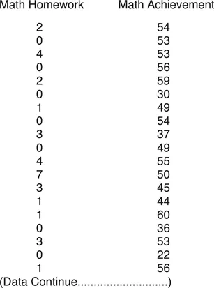
A portion of the data is shown in Figure 1.1. The complete data are on the website that accompanies this book, www.tzkeith.com, under Chapter 1, in several formats: as an SPSS System file (homework & ach.sav), as a Microsoft Excel file (homework & ach.xls), and as an ASCII, or plain text, file (homework & ach.txt). The values for time spent on Math Homework are in hours, ranging from zero for those who do no math homework to some upper value limited by the number of free hours in a week. The Math Achievement test scores have a national mean of 50 and a standard deviation of 10 (these are known as T scores, which have nothing to do with t tests).²

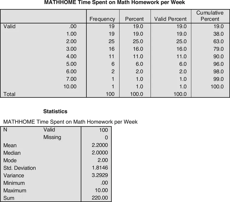
Let’s turn to the analysis. Fortunately, you have good data analytic habits: you check basic descriptive data prior to doing the main regression analysis. Here’s my rule: Always, always, always, always, always, always check your data prior to conducting analyses! The frequencies and descrip tive statistics for the Math Homework variable are shown in Figure 1.2. Reported Math Home work ranged from no time, or zero hours, reported by 19 students, to 10 hours per week. The range of values looks reasonable, with no excessively high or impossible values. For example, if someone had reported spending 40 hours per week on Math Homework, you might be a little suspicious and would check your original data to make sure you entered the data correctly (e.g., you may have entered a “4” as a “40”; see Chapter 10 for more information about spotting data problems). You might be a little surprised that the average amount of time spent on Math Homework per week is only 2.2 hours, but this value is certainly plausible. (As noted in the Preface, the regression and other results shown are portions of

Figure 1.1 Portion of the Math Homework and Achievement data. The complete data are on the website under Chapter 1.

Figure 1.2 Frequencies and descriptive statistics for Math Homework.

an SPSS printout, but the information displayed is easily generalizable to that produced by other statistical programs.)

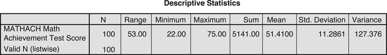
Next, turn to the descriptive statistics for the Math Achievement test (Figure 1.3). Again, given that the national mean for this test is 50, the 8th-grade school mean of 51.41 is reasonable, as is the range of scores from 22 to 75. In contrast, if the descriptive statistics had shown a high of, for example, 90 (four standard deviations above the mean), further investigation would be called for. The data appear to be in good shape.

The Regression Analysis

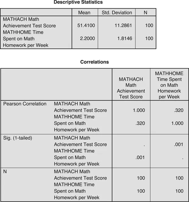
Next, we conduct regression: we regress Math Achievement scores on time spent on Homework (notice the structure of this statement: we regress the outcome on the influence or influences). Figure 1.4 shows the means, standard deviations, and correlation between the two variables.

Figure 1.3 Descriptive statistics for Math Achievement test scores.

Figure 1.4 Results of the regression of Math Achievement on Math Homework: descriptive statistics and correlation coefficients.

The descriptive statistics match those presented earlier, without the detail. The corre lation between the two variables is .320, not large, but certainly statistically significant (p < .01) with this sample of 100 students. As you read articles that use multiple regression, you may see this ordinary correlation coefficient referred to as a zero-order correlation (which distinguishes it from first-, second-, or multiple-order partial correlations, topics discussed in Appendix C).

Next, we turn to the regression itself; although we have conducted a simple regres sion, the computer output is in the form of multiple regression to allow a smooth transition. First, look at the model summary in Figure 1.5. It lists the R, which normally is used to des ignate the multiple correlation coefficient, but which, with one predictor, is the same as the simple Pearson correlation (.320).³ Next is the R², which denotes the variance explained in the outcome variable by the predictor variables. Homework time explains, accounts for, or predicts .102 (proportion) or 10.2% of the variance in Math test scores. As you run this regression yourself, your output will probably show some additional statistics (e.g., the adjusted R²); we will ignore these for the time being.

Is the regression, that is, the multiple R and R², statistically significant? We know it is, because we already noted the statistical significance of the zero-order correlation, and this “multiple” regression is actually a simple regression with only one predictor. But, again, we’ll check the output for consistency with subsequent examples. Interestingly, we use an F test, as in ANOVA, to test the statistical significance of the reg...