Using R for Bayesian Spatial and Spatio-Temporal Health Modeling

Andrew B. Lawson

• Publisher: Chapman and Hall/CRC
• Year: 2021
• Print ISBN: 9780367490126
• eBook ISBN: 9781000376722
• Edition: 1
• Topic: Mathematics
• Subtopic: Programming Languages
• Index: Mathematics

Progressively more and more attention has been paid to how location affects health outcomes. The area of disease mapping focusses on these problems, and the Bayesian paradigm has a major role to play in the understanding of the complex interplay of context and individual predisposition in such studies of disease. Using R for Bayesian Spatial and Spatio-Temporal Health Modeling provides a major resource for those interested in applying Bayesian methodology in small area health data studies.

Features:

• Review of R graphics relevant to spatial health data

• Overview of Bayesian methods and Bayesian hierarchical modeling as applied to spatial data

• Bayesian Computation and goodness-of-fit

• Review of basic Bayesian disease mapping models

• Spatio-temporal modeling with MCMC and INLA

• Special topics include multivariate models, survival analysis, missing data, measurement error, variable selection, individual event modeling, and infectious disease modeling

• Software for fitting models based on BRugs, Nimble, CARBayes and INLA

• Provides code relevant to fitting all examples throughout the book at a supplementary website

The book fills a void in the literature and available software, providing a crucial link for students and professionals alike to engage in the analysis of spatial and spatio-temporal health data from a Bayesian perspective using R. The book emphasizes the use of MCMC via Nimble, BRugs, and CARBAyes, but also includes INLA for comparative purposes. In addition, a wide range of packages useful in the analysis of geo-referenced spatial data are employed and code is provided. It will likely become a key reference for researchers and students from biostatistics, epidemiology, public health, and environmental science.

1

Introduction and Datasets

Bayesian spatial health modeling, sometimes also known as Bayesian disease mapping, has matured to the extent that a range of computational tools exist to enhance end user’s ability to analyze and interpret the variations in disease risk commonly found in human and animal populations. This has been enhanced by the easy availability of geographical information systems (GIS) such as ArcGIS or Quantum GIS (QGIS). While a variety of software platforms host specialist programs, there is now a large body of software available for the R programming environment, and given the general accessibility of this free software platform it is advantageous to consider the integration of analyses on this platform. A range of Bayesian modeling software is now available on R which can be used for spatial health modeling. Within R, it is possible to process geo-referenced data, including GIS-based information such as adjacency of regions and polygon neighborhoods. With the standard capabilities of R for descriptive statistics and R’s extensive plotting facilities, it is easy to explore geo-referenced data.

With the addition of a range of packages that can fit Bayesian Hierarchical models (BHMs) it is now possible to carry out both exploration and analysis of spatial health data in one environment. In addition, a selection of packages that fit BHMs can also fit spatial dependence structures and so address different kinds of spatial confounding of risk. This means that state-of-the-art models can be fitted and analyzed.

Estimation in Bayesian HMs is based on a parameter posterior distribution, which is a function of a data likelihood and prior distributions for model parameters. Bayesian HMs are often relatively sophisticated and require approximation methods to address parameter estimation. Two major approaches to this approximation are commonly found: (1) posterior sampling where an iterative algorithm is used to provide a sample of parameter values that can be summarized to yield estimates, (2) numerical approximation to an integral, based on an approximate form of the posterior distribution. Posterior sampling is often carried out using Monte Carlo methods and a set of methods called Markov chain Monte Carlo (McMC) have been developed to facilitate this estimation approach. Essentially in this approach the posterior distribution is approximated by samples, and sampled values are used to summarize the posterior quantities of interest (such as mean, variance etc). Numerical approximation of the posterior distribution commonly involves a Laplace approximation which matches a Gaussian distribution to the form of the posterior distribution and provides estimates based on this approximation. Numerical approximation can be computationally advantageous especially in large-scale problems (big data) where sampling becomes inefficient. On the other hand McMC can provide a large amount of information concerning the form of the posterior distribution, which is not usually available immediately from numerical approximation.

For the application of BHMs to disease mapping, there is an extensive literature now available (e.g., Breslow and Clayton, 1993; Besag et al., 1991; Leroux et al., 2000; Blangiardo et al., 2013 and Lawson, 2018 for a review). Often, this area is termed Bayesian Disease Mapping (BDM) and this acronym will be used extensively here. A major issue that arises when considering the model-based approach to disease mapping is the assumption of the spatial continuity of risk. Disease risk, as displayed as incidence in small areas, is dependent on the underlying population at risk of the disease. As this population is discrete in nature, in that subjects must exist for disease to occur, then disease risk will also be discrete. At the individual level a subject will have a binary outcome (disease/no disease) and when aggregated to a population then a count of disease arises. At the finest spatial scale an individual subject could have an address location associated with them. This could be a residential address for a person or a farm for an animal (say). Essentially the location is a unique identifier. At this scale the location is stochastic and a point process of cases and controls will arise. Once aggregated to arbitrary small areas (census tracts, post codes, provinces, etc.) then counts within areas of cases, and of controls, will arise. Often, if the population is large relative to the probability of disease, i.e., in the case of a relatively rare disease, then a Poisson count data model for the cases is often assumed. When a smaller finite population occurs then a binomial model is more appropriate with case count modeled in relation to the case plus control total population. These data models which assume independent contributions from each subject can be justified based on conditional independence within the BHM hierarchy.

Although populations are discrete, it is also the case that a choice of risk model can be made whereby components of risk are assumed to be continuous. For example, it is reasonable to assume that environmental stressors such as pollution levels are spatially and temporally continuous. Often BDM models consist of fixed (predictor) effects and random effects. These represent observed outcome confounders and unobserved confounding respectively. The choice of random effect to model unobserved confounding can lead to markedly different model paradigms. If the unobserved correlated confounding is continuous then it would be justified to consider continuous spatial/temporal random effects (such as spatial/temporal Gaussian processes). However, instead, it is more usual to assume Markov random field (MRF) models, whereby only local neighborhood dependence defines the correlated effect. Given the discrete nature of small areas, this would usually seem to be a natural approach.

In this work both spatial BDM models and spatio-temporal examples will be considered. Spatio-temporal (ST) data arises naturally in disease mapping studies, as all cases of disease have associated a date and/or time of diagnosis. Aggregation of cases into time periods and small areas leads to spatio-temporal count sequences. Spatial BDM models can be extended relatively easily to deal with ST data in the form of counts in time periods and small areas. Special models can be developed for ST data variants, such as spatial survival modeling, spatial recurrent event, or longitudinal modeling.

To set the scene with respect to historical development, a brief, and by no means exhaustive, overview of the development of approaches to BDM is presented here. Early examples of Bayesian models were (Clayton and Kaldor, 1987) using empirical Bayes approximation, the use of MRF models for (transformed) counts include Cressie and Chan (1989), Bayesian Poisson data models with conditional autoregressive random effects and MCMC (Besag et al., 1991), space-time models (Bernardinelli et al., 1995; Waller et al., 1997; Knorr-Held, 2000). Some more recent developments with special focus are: (a) multivariate disease mapping (Gelfand and Vounatsou, 2003, Jin et al., 2005; Jin et al., 2007; Martinez-Beneito et al., 2017), (b) spatial survival modeling (Osnes and Aalen, 1999; Henderson et al., 2002; Banerjee et al., 2003; Cooner et al., 2006; Zhou et al., 2008; Lawson and Song, 2009; Banerjee, 2016; Onicescu et al., 2017b; Onicescu et al., 2017a), (c) spatial longitudinal modeling (Lawson et al., 2014), and (d) infectious disease modeling (Sattenspiel and Lloyd, 2009; Lawson and Song, 2010; Chan et al., 2010; Lawson et al., 2011; Corberán-Vallet, 2012).

Bayesian hierarchical modeling (BHM) often requires sophisticated numerical methods to be employed to provide estimates of relevant parameters. To this end, software packages have been developed on the R platform that either implement posterior sampling via MCMC, or numerical integration using Laplace approximation. While a number of variants exist of these main computational approaches, in this work the focus is on the main packages which implement posterior sampling and Laplace approximation for BDM. These consist of WinBUGS/OpenBUGS, nimble, CARBayes, which use posterior sampling. STAN and jags are not implemented here as they have been used less frequently. Jags does not have spatial prior distributions and STAN only recently implemented these models (see e.g., package brms and the cor_car function, Morris et al., 2019). For numerical approximation, the Laplace approximation as implemented in the R-INLA package is reviewed.

This work is closely tied to the preceding volume on Bayesian Disease Mapping by Lawson (2018). The intention with this work is to provide direct exposure to the software that can be used to implement BHMs in the context of disease mapping. To this end, detailed discussion of models and their justification is not attempted, but reference is made to book sections in Lawson (2018) where the models and computational approaches are described in more detail. In addition, as a cloud resource a variety of examples of model code in different forms (BUGS, INLA, nimble, CARBayes) are available on GitHUB: https:/​/​github.com/​Andrew9Lawson. Two different branches can be found at this site. A nimble code branch and other software branch (OpenBUGS, INLA, CARBayes). Examples used in this work can also be found at this site. Additional resources can also be found at http:/​/​people.musc.edu/​∼abl6/​. The software version of R used in this work is 3.6.2.

1.1 Datasets

Here, I describe the basic datasets that will be analyzed in this work. As a comparison of software is to be made I have limited the range of datasets to a small number so that direct comparison is facilitated.

Spatial data

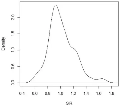
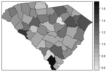
(1) All ICD code respiratory cancers at county level in South Carolina, USA, for the year 1998. This represents a broad spectrum of etiology and while risk is relatively low the counts are not sparse (i.e., no zero counts in counties). The data consist of counts of cases and expected rates computed from the statewide population rate. I assume indirect standardization. The standardized incidence ratio (SIR) is computed from the ratio : count/expected rate. Figure 1.1 displays the marginal density estimate of the standardized incidence ratio. Figure 1.2 displays the mapped SIR for these data.

Figure 1.1
Standardized Incidence ratio for all respiratory cancers in South Carolina counties in 1998: marginal density estimate using a default bandwidth.

Figure 1.2
Standarized incidence ratio for all respiratory cancers in 1998, South Carolina counties, USA.

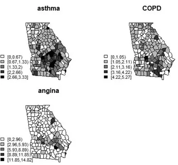
(2) Multivariate example: asthma, COPD, and angina incidence in counties of Georgia, USA for the year 2005. These data were originally analyzed in Lawson (2018), Chapter 10. These data are considered to possibly be correlated in that their spatial incidence distribution may show similar clustering or other artifacts of disease incidence. Figure 1.3 displays the SIRs (relative risk estimates) for the incidence of these respiratory and coronary outcomes in the counties of Georgia USA for year 2005. The expected rates were calculated from statewide incidence rate for each disease separately.

Figure 1.3
Relative risks (SIRs) for asthma, COPD, and angina incidence in the state of Georgia, USA, for the year 2005.

(3) Low birth weight and very low birth weight events in 2007 in the counties of Georgia USA. This example includes an aggregate count outcome with a binomial model with 5 predictors and is featured in the variable selection section of Chapter 16. This is used as an example of aggregate-level regression where selection of variables is a focus.

(4) Cross-sectional time period (single biweekly) of foot and Mouth disease (FMD) within parishes during the epidemic in North West England in 2001. Counts of infected premises are available as well as total numbers of premises. Figure

Spatio-temporal data

Outcomes in the form of counts within small areas associated with a sequence of discrete time periods are also often a focus of analysis. In this situation the focus is usually on both spatial, temporal, as well as spa...

Table of contents

• Cover
• Half Title
• Title Page
• Copyright Page
• Contents
• Preface
• Biography
• List of Tables
• 1 Introduction and Datasets
• 2 R Graphics and Spatial Health Data
• 3 Bayesian Hierarchical Models
• 4 Computation
• 5 Bayesian model Goodness of Fit Criteria
• 6 Bayesian Disease Mapping Models
• I Basic Software Approaches
• II Some Advanced and Special topics
• References
• Index