JMP for Mixed Models

Ruth Hummel, Elizabeth A. Claassen, Russell D. Wolfinger

• Publisher: SAS Institute
• Year: 2021
• Print ISBN: 9781951684020, 9781952365218
• eBook ISBN: 9781952363856
• Topic: Informatica
• Subtopic: Informatica generale

Discover the power of mixed models with JMP and JMP Pro.

Mixed models are now the mainstream method of choice for analyzing experimental data. Why? They are arguably the most straightforward and powerful way to handle correlated observations in designed experiments. Reaching well beyond standard linear models, mixed models enable you to make accurate and precise inferences about your experiments and to gain deeper understanding of sources of signal and noise in the system under study. Well-formed fixed and random effects generalize well and help you make the best data-driven decisions.

JMP for Mixed Models brings together two of the strongest traditions in SAS software: mixed models and JMP. JMP's groundbreaking philosophy of tight integration of statistics with dynamic graphics is an ideal milieu within which to learn and apply mixed models, also known as hierarchical linear or multilevel models. If you are a scientist or engineer, the methods described herein can revolutionize how you analyze experimental data without the need to write code.

Inside you'll find a rich collection of examples and a step-by-step approach to mixed model mastery. Topics include:

• Learning how to appropriately recognize, set up, and interpret fixed and random effects
• Extending analysis of variance (ANOVA) and linear regression to numerous mixed model designs
• Understanding how degrees of freedom work using Skeleton ANOVA
• Analyzing randomized block, split-plot, longitudinal, and repeated measures designs
• Introducing more advanced methods such as spatial covariance and generalized linear mixed models
• Simulating mixed models to assess power and other important sampling characteristics
• Providing a solid framework for understanding statistical modeling in general
• Improving perspective on modern dilemmas around Bayesian methods, p-values, and causal inference

Chapter 1

Introduction

1.1 What is a Mixed Model?

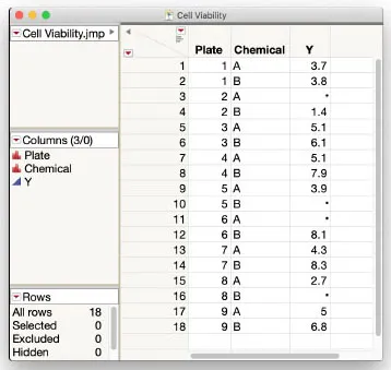
Imagine you are lab scientist studying the effect of two chemicals, A and B, on cell viability. You prepare nine plates of media with healthy cells growing on each, and then apply A and B to randomly assigned halves of each plate. After a suitable incubation period, you collect treated cells from the halves of each plate and perform an assay on each sample to compute a measurement Y of interest. Four of the samples are accidentally contaminated during processing and produce no assay results. Your data table in JMP looks like Figure 1.1.

How should you analyze these data? A primary goal is to estimate the causal effect of Chemical on Y, while taking appropriate account of the experiment design based on Plate. A standard way to begin is to formulate a statistical model of Y as a function of Chemical and Plate. A statistical model is a mathematical equation formed using parameters and probability distributions to approximate a data-generating process. We refer to Y as the response in the model, or alternatively as the dependent variable or target. We refer to Chemical and Plate as factors or independent variables.

Note the different natures of Chemical and Plate. Chemical has two specifically chosen levels, A and B, whereas the levels of Plate are effectively a random set of such plates you routinely make in your lab. This is a most basic example of a case in which you would want to use a mixed model, which is a statistical model that includes both fixed effects and random effects. Here Chemical would be considered a fixed effect and Plate a random effect.

Figure 1.1: Cell Viability Data

Key Terminology

Fixed Effect A statistical modeling factor whose specific levels and associated parameters are assumed to be constant in the experiment and across a population of interest. Scientific interest focuses on these specific levels. For example, when modeling results from three possible treatments, your focus is on which of the three is best and how they differ from each other.

Random Effect A statistical modeling factor whose observed values are assumed to arise from a probability distribution, typically assumed to be normal (Gaussian). Random effects can be viewed as a random sample from a population that forms part of the process that generates the data you observe. You want to learn about characteristics of the population and how it drives variability and correlations in your data. You want inferences about fixed effects in the same model to apply to the population corresponding to this random effect. You may also want to estimate or predict the realized values of the random effects.

Mixed Model A statistical model that includes both fixed effects and random effects.

Why is the distinction between fixed and random effects important? Many, if not most, real-life data sets do not satisfy the standard statistical assumption of independent observations. In the example above, we naturally expect observations from the same plate to be correlated as opposed to those from different plates. Random effects provide an easy and effective way to directly model this correlation and thereby enable more accurate inferences about other effects in the model. In the example, specifying Plate as a random effect enables us to draw better inferences about Chemical. Failure to appropriately model design structure such as this can easily result in biased inferences. With an appropriate mixed model, we can estimate primary effects of interest as well as compare sources of variability using common forms of dependence among sets of observations.

The use of fixed and random effects have a rich history, with countless successful applications in most every major scientific discipline over the past century. They often go by several other names, including blocking models, variance component models, nested and split-plot designs, hierarchical linear models, multilevel models, empirical Bayes, repeated measures, covariance structure models, and random coefficient models. They also overlap with longitudinal, time series, and spatial smoothing models. Mixed models are one of the most powerful and practical ways to analyze experimental data, and if you are a scientist or engineer, investing time to become skilled with them is well worth the effort. They can readily become the most handy method in your analytical toolbox and provide a foundational framework for understanding statistical modeling in general.

This book builds on the strong tradition of mixed model software offered by SAS Institute, beginning with PROC VARCOMP and PROC TSCSREG in the 1970s, to PROC MIXED, PROC PHREG, PROC NLMIXED, and PROC PANEL in the 1990s, PROC GLIMMIX in the 2000s, and more recently PROC HPMIXED, PROC LMIXED, PROC MCMC, PROC BGLIMM, and related Cloud Analytic Service actions in SAS Viya. We borrow extensively from SAS for Mixed Models by Littell et al. (2006) and Stroup et al. (2018). Mixed model software in various forms has evolved extensively and somewhat independently over the past several decades in other packages including R (lme4, lmer, nlme), SPSS Mixed, Stata xtmixed, HLM, MLwiN, GenStat, ASREML, MIXOR, WinBUGS/OpenBUGS, Stan, Edward, Tensorflow Probability, PyMC, and Pyro (web search each for details). The existence and popularity of all of these also speaks to the power and usefulness of mixed model methodology. Some differences in syntax, terminology, and philosophy naturally occur between the various implementations, and we hope the explanations and coverage in this book are clear enough to enable translation to other software should the need arise.

Mixed model functionality has been available in JMP since 2000 (JMP 4), and a dedicated mixed model personality in Fit Model was released in 2013 (JMP Pro 11). It continues to be an area of active development. The unique and powerful point-and-click interface of JMP, designed intrinsically around dynamic interaction between graphics and statistics, makes it an ideal environment within which to fit and explore mixed models. Analyzing mixed models in JMP offers some natural conveniences over any approach that requires you to write code, especially with regards to the engaging interplay between numerical and pictorial results of statistical modeling. To get an initial idea of how it works, let’s dive right into our first mixed model analysis in JMP.

1.2 Cell Viability Example

Consider the cell viability data shown the previous section and contained in Cell Viability.jmp.

Using JMP

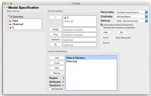
With the Cell Viability table open and active, from the top menu bar click Analyze > Fit Model to bring up a dialog box. On the left side, choose Y, then assign it to the Y role. Make sure the Standard Least Squares personality is selected in the upper right corner. Then select Chemical and Plate, and click Add to assign them to the Construct Model Effects box. In that box, select Plate, then click the red triangle

beside Attributes and select Random Effect. You will see "& Random" added beside Plate in the box, confirming designation as a random effect. Click Run to fit the model.

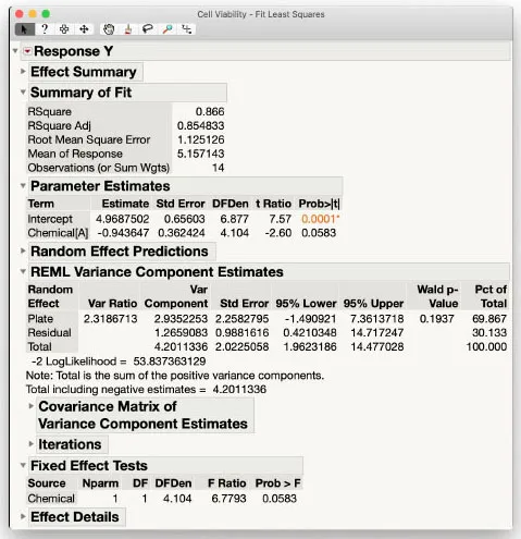
The model fitting results in Figure 1.2 are comprehensive with numerous statistics and details. We only focus on a few of the most important ones here and explore others in more depth in later chapters.

Figure 1.2: Mixed Model Results for Cell Viability Data

In the Parameter Estimates box in Figure 1.2, the row beginning with "Chemical[A]" contains the estimate of the effect of Chemical A (-0.94) along with its estimated standard error (0.36). Note this standard error is computed accounting for the random effect Plate in the model. Taking the ratio of these two numbers produces a t-statistic (signal-to-noise ratio) of -2.60. The associated p-value is 0.058, just above the classical 0.05 rule of thumb for statistical significance. As emphasized in recent commentary (see The American Statistician (2019)), such a borderline “non-significant” result should be interpreted in conjunction with the effect estimate itself and how it relates to estimated levels of variability in the context of the experiment.

Not shown is the estimate of Chemical B, which is automatically set equal to the negative of Chemical A in order to identify the model using the traditional sum-to-zero parameterization for linear models. The statistics for Chemical B are therefore identical to those from Chemical A, but the main effect and t-statistic have opposite signs. Our main conclusion is that Chemical B is estimated to have an overall effect around 1.9 units higher than Chemical A.

The REML Variance Component Estimates box provides estimates of the variance components along with associated statistics. Here we see that the estimate of plate-to-plate variability is 2.3 times larger than within-plate (residual error) variability. Such a result speaks to the two primary sources of random variability in this experiment and prompts questions as to why plates are varying to this degree.

Key Terminology

The acronym REML refers to restricted (or residual) maximum likelihood, the best-known method for fitting mixed models assuming that any missing data are missing at random, and equivalent to full information maximum likelihood from econometrics. Refer to Stroup et al. (2018) for details and theory behind REML in mixed models.

All of the mixed model results help to answer various aspects of research questions involving these chemicals and the assay used t...

Table of contents

• Cover
• Copyright Page
• Contents
• About This Book
• About the Authors
• Acknowledgements
• 1 Introduction
• 2 ANOVA with a Single Blocking Effect
• 3 Models with Factorial Treatment Designs
• 4 Multiple Random Effects
• 5 Regression, Random Coefficients, and Multilevel Models
• 6 Repeated Measures and Longitudinal Data
• 7 Spatial Models
• 8 Simulation and Power Analysis
• 9 Generalized Linear Mixed Models
• 10 Mixed Models Amidst Modern Debates
• A List of Examples Used in This Book