Escape Velocity

Better Metrics for Agile Teams

Doc Norton

• Publisher: OnBelay Consulting, LLC
• Year: 2020
• eBook ISBN: 9780578644851
• Edition: 1
• Topic: Computer Science
• Subtopic: Software Development
• Index: Computer Science

Velocity is the most commonly used metric in agile software delivery. It is also perhaps the least effectivemetrics in agile software delivery. In "Escape Velocity", Doc Norton walks the reader through common issues with metrics and how to avoid them, altermative metrics that not only help agile teams perform better, but enable them to continuously improve, and techniques for forecasting that vastly outperform the use of velocity. In a quirky, casual, and information dense style, Doc Norton makes the topic of tracking data entertaining and shows us how to be more effective in the pursuit of excellent software.

Other Metrics

So I think we’ve made the case against Velocity as a metric. And we’ve given you some things to think about as you’re considering what metrics to use instead (if any). Now let’s take a look at some other metrics that might help you get to the root cause of team issues, help you figure out when things will actually be done, and help you figure out if you’re doing a quality job - from a technical and customer perspective.

Lead Time

In software development Lead Time is generally considered the time elapsed from the moment a request is received to the moment that same request is available in production. I call this the time from, “Hey, wouldn’t it be nice if..?”, to, “Hey, ain’t that nice?”

Lead and Cycle Time

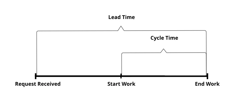
For some teams, lead time is measured from when the team starts to look at the request. In these cases, the timer doesn’t start when an item hits the backlog, but rather when the item gets picked up for analysis, or whatever is the initial step in the process. For our purposes, we are going to consider lead time to be from the moment a request is pulled from the backlog to be worked on. We’re not going to concern ourselves with the amount of time an item sits in the backlog, as this has more to do with the volume of items and prioritization than it does with actual throughput and team capability.

Tracking the production lead time (time from work starting to in production) allows us to produce better projections for when an item will be complete. If we know there are seven items in the backlog ahead of this one with three items in progress for a total of 10 items ahead of this one and we know that on average an item takes 2 days from commencement to completion, we can reasonably estimate that this one will be done in 20 days. Sort of.

At first blush, an average seems perfectly reasonable for estimations. Essentially half of the items will complete sooner than the average and half of the items will complete later than the average with some amount falling precisely on the average. What we’ve just described here is a normal distribution, which when graphed results in what is often called a bell curve. With a normal distribution, if you use the average to estimate, you have a 50:50 shot of being right.

But you don’t have a 50:50 shot of being right when you use the average lead time. Lead times don’t happen on a perfect bell curve.

Lead Time Distributions

Take a moment and think about a trip you take regularly. This might be your commute to or from work. Maybe it is visiting a family member.

For me, this is my commute to the client every day. For the past several months, I’ve been working with one primary client as we help them transition toward an experimentation mindset with a focus on flow and valuable outcomes.

I drive to the client from a nearby hotel. On average, that commute takes 10 minutes. Most mornings I catch at least one light or get behind someone doing 25 in a 40 for a mile or two. Some mornings, the lights are in my favor and the slow pokes stay out of my way. On such days, I can get from hotel to client in about 7.5 minutes. Under no legal circumstances can I get to the client faster than in seven minutes. Account for distance and general safety, and seven minutes is already pushing it; possible, but not likely. Under no physical circumstances can I get to the client faster than in five minutes. Even if I ignore all laws of man, the laws of physics still bind me.

On the other end of the spectrum, however, the commute can take (and has taken) much longer. For a couple of weeks, the main thoroughfare was under construction, reducing traffic to a single lane in the outbound direction on a road that is normally three lanes. One morning, there was an unusual amount of traffic and things got jammed up, causing everything to move quite slowly. People snuck out into intersections in hopes of slipping through before the light changed. Some didn’t make it and the resulting jam caused people coming from perpendicular roads to do the same; stay in the intersection in hopes of making it through after things cleared. Basically, we were down to about two or three cars per direction clearing the intersection for every complete turn of the light.

I got stuck in a long line of traffic and with the other road closings and single lane restrictions, I had nowhere to go but forward. The light did a full rotation once every 6 minutes. There were approximately 15 cars in front of me. 27 minutes later, I cleared the light and finally arrived at the client a full 38 minutes after I’d left the hotel.

Let’s imagine that I’d tracked my morning commute time to work each day and I recorded it on a sheet. And for the sake of this example, let’s further imagine that my 38 minute outlier day had not yet occurred. That sheet might have looked something like this:

Morning Commute

Mon	Tue	Wed	Thu	Fri
10.25	9.5	9.75	10	12.25
10	15.25	12.5	10.75	9.25
10.25	10.25	9	10.5	10.25
10.5	10.75	13.75	11	11.25
14	12	10.5	13	10.25
11.25	13.5	11.5	14.25	10.25

The data shows us that while the trip can take no less then nine minutes, it can take as much as 15.25 minutes with an average trip time of 11.25 minutes. Our shortest trip is 2.25 minutes quicker than average. Whereas our longest trip is four minutes slower than average. And as we indicated, no matter how hard we try to get there sooner, we are ultimately bound by the laws of physics. But on the other end, in terms of how long the trip can take, we are pretty much bound only by the laws of reason.

Now, if you asked me how long it took me to get to work, I might say, “Between nine and fifteen minutes.”, and I’d be accurate, but not precise. I could also say, “11.25 minutes on average,” which is precise, but not necessarily accurate. But what if you were asking me to guarantee I could make it to work within the time I estimate? What if you were asking me to make a commitment and to guarantee with 100% certainty that I could get to work within the time committed? Does this sound familiar to you? Doesn’t this sound like just about every “estimation” discussion you’ve ever had at work? Well, if this were the case, then based on the data available to me, I’d have to say, “I can get to work within 15.25 minutes.”

A lot of people would say I am padding. But I am not padding. I am providing a 100% guarantee based on the data available. Which is what I was asked for.

Some would say I am gaming the system. More often that not, I make it to work in under 11 minutes. How could I possibly think an estimate of 15.25 minutes is reasonable? That’s more than 25% padding on top of the average for something as simple as driving to work; same car, same driver, same route - every day.

But the reasonableness of my estimate is the wrong question, now isn’t it? The right question is how could one possibly expect, in a system with such variability, that anyone could make a commitment they will be held accountable to and use a low probability number?

Low probability? What do I mean by a low probability number?

Well, let’s look at the data again. This time, let’s look at it on a distribution graph.

Lead Time Distribution for Drive Time

So far, so good. This is probably what you’d expect to see. A cluster of numbers near the low end with a peak around the average and a longer tail. This is a right-skewed distribution. Remember when we talked about how lead time doesn’t happen on a perfect bell curve? For similar reasons to our commute, lead times for software development also happen on a right-skewed distribution. The term right-skewed indicates that the graph can trail off to the right for a significant distance. This is also referred to as a positively skewed distribution graph. In a distribution graph, our X axis represents increments increasing in value from left to right. So a tail that points right, points in the positive direction. Correspondingly a tail that points to the left, points in the negative direction.

Okay, so right-skewed distribution. Great. But what do I mean when I say a number is a low probability number? And why did I say the average was a low probability number?

Let’s draw a line on the graph at the mean, or numerical average.

Lead Time Distribution for Drive Time with Mean

We can now see that 19 of the data points fall on or before the mean, while 11 of the data points fall after the mean. So if we were to use the mean (or average) as our commitment, the data tells us we have a 65.5% chance of hitting or bettering the commitment. That means we have a 34.5% chance of missing it. Or a one in three chance of going over our commitment.

So our probability for this estimate is roughly 66%. We expect to be over the estimate 33% of the time AND we expect to be under the estimate 62% of the time. We expect to actually hit the estimate, 3.4% of the time.

In most organizations, an estimate that we think we’ll overshoot 33% of the time would be considered a low probability estimate. Certainly if there is gnashing of teeth when the estimate is...

Table of contents

• Title Page
• Table of Contents
• Dedication
• About
• Preface
• What is Velocity?
• Velocity Anti-Patterns
• Potential Side Effects of Metrics
• Variable Velocity
• Other Metrics
• Customer Metrics
• Looking for Correlations
• Balanced Metrics
• Acknowledgements
• Notes