Water Environment Modeling

Clark C.K. Liu, Pengzhi Lin, Hong Xiao

• Publisher: CRC Press
• Year: 2021
• ISBN:
  9781000469851
• Edition: 1
• Topic: Tecnologia e ingegneria
• Subtopic: Gestione ambientale

Water Environment Modeling covers the formulations and applications of mathematical models that simulate water flow and chemical transport in rivers, lakes, groundwater, estuaries, coastal, and ocean waters. These models are used to evaluate the response of water environment to human interventions and serve as useful analytical tools for water pollution control and resource management.

Simple and comprehensive modeling techniques and their practical applications are presented with examples and exercises, most of which are derived from actual case studies. In general, simple models can be solved analytically and comprehensive models require numerical solutions. While simple models are usually adopted for preliminary assessment of a particular water environment, comprehensive models are used to provide detailed spatial and temporal variations of pollutants in complex environments. The system-based models in the forms of integral equations are introduced as an alternative modeling approach.

This textbook is ideal for advanced undergraduate students and graduate students in civil and environmental engineering and related academic fields. It is also suitable as a reference book for practicing engineers and scientists.

Authors:

Clark C.K. Liu is Emeritus Professor of the Department of Civil and Environmental Engineering at University of Hawaii and former Environmental Engineering Director of US National Science Foundation.

Pengzhi Lin is Professor of State Key Laboratory of Hydraulics and Mountain River Engineering at Sichuan University. He is the author of Numerical Modeling of Water Waves (CRC Press, 2008).

Hong Xiao is Professor and Vice Director of Hydroinformatics Institute of the State Key Laboratory of Hydraulics and Mountain River Engineering at Sichuan University.

Chapter 1
Introduction

DOI: 10.1201/9781003008491-1

1.1 WATER RESOURCES AND WATER QUALITY MANAGEMENT

1.1.1 Hydrologic cycle

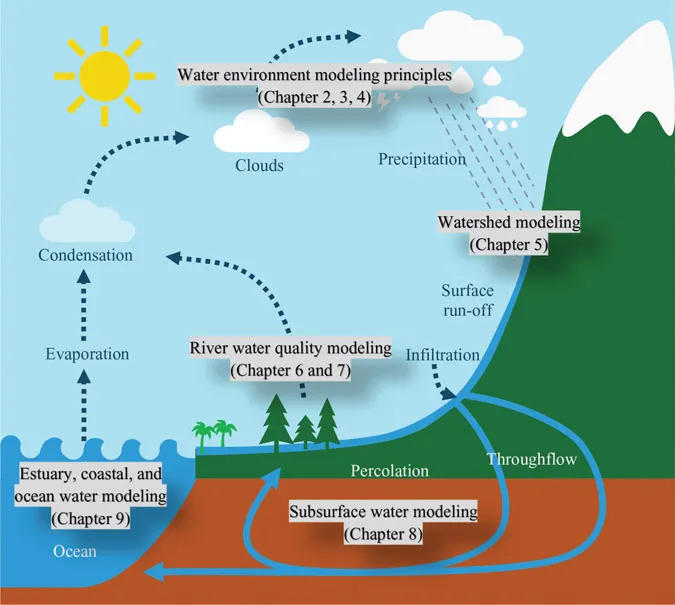
The hydrologic cycle, which describes the journey and balance of water on the earth’s surface, below the ground, in the atmosphere, and back again (Figure 1.1), is an important concept in the discussion of generation, development, and protection of water resources.

Figure 1.1 Hydrologic cycle and the scope of water environment modeling.

Although the hydrologic cycle has neither a beginning nor an end, in order to discuss its components clearly, we usually start the cycle from evapotranspiration, which is the sum of evaporation from the land surface plus transpiration from plants. Water vapor that enters the atmosphere through the evapotranspiration processes condenses to form clouds. Under suitable conditions, tiny water droplets in the cloud further condense to form precipitation and return to the ground. It should be noted that precipitation includes rain, snow, hail, and so on. For convenience of discussion, it is collectively referred to as rain in this book.

The rain wets the soil and then begins to infiltrate into the underground. The infiltration rate varies with soil properties and land uses. For example, it can reach above 300 mm/h in forests, approximately 30 mm/h on farmlands, and even much lower in cities.

Overland runoff occurs when the rain rate exceeds the infiltration rate. As the infiltrated water enters the upper unsaturated soil, the water content increases. The water continues to flow slowly downward into the saturated layer, becoming groundwater and flowing slowly to the outflow area. The groundwater outflow area includes mountainous springs, riverbeds and lake bottoms, and seeps near the sea.

After the water enters rivers and lakes through the surface runoff and groundwater flow process, it continues to flow into the ocean. Evapotranspiration brings water back into the atmosphere from rivers, lakes, and oceans, completing the hydrologic cycle.

The two components, evapotranspiration and precipitation, in the hydrologic cycle can be viewed as a huge desalination project. The energy required to drive this project comes from solar radiation. The total amount of solar radiation energy received by the Earth is about 2.0 million TW (10¹² W), of which 1.2 million TW reaches the ground, as presented in Table 1.1.

Table 1.1 Solar radiation energy that drives the hydrologic cycle

Energy Distribution	Value (TW)
Solar radiation energy received by the earth	2.0 million
Solar radiation energy reaching the ground	1.2 million
Energy consumed by evapotranspiration	400,000
Energy lost in the river	80
Energy converted into hydropower	1

One-third of the solar radiation energy that reaches the ground (400,000 TW) is consumed by the evapotranspiration process of the hydrologic cycle (Overman, 1969), while the total energy consumption by the world population is about 18 TW (International Energy Agency, 2015). Table 1.1 also shows that the global energy loss from rivers to oceans is about 80 TW, among which less than 1 TW has been converted into hydropower. Building dams to develop hydropower can alter the ecological environment; therefore, further massive hydropower development is limited. Energy–water nexus is one of the biggest problems faced by mankind in the 21st century.

As analytical tools in managing water resources and conserving ecological environment, water environment models are of great importance in meeting the challenge of energy–water nexus.

When water evaporates from the earth’s surface, it absorbs heat and reduces ambient temperature, whereas it releases heat and increases temperature when it condenses. Therefore, the hydrologic cycle is closely related to the climate. Various economic activities of human beings in the modern era have greatly changed the solar radiation energy absorbed by the earth’s surface, resulting in the problem of global warming. Global warming not only increases the average temperature on the earth but also changes the temporal and spatial distribution of global precipitation, which has a great impact on the development and management of water resources.

1.1.2 Distribution of freshwater resources on the earth

A large amount of water flows in different components of the hydrologic cycle, and its total volume is difficult to calculate precisely. Table 1.2 lists the estimated values that are commonly cited. Tm³, a huge volume unit, is used in the table. One Tm³ is equal to one million Mm³, one Mm³ is equal to one million cubic meters, and one cubic meter is equal to 1,000 liters. Table 1.2 shows that the total annual rainfall on the land is 120 Tm³, and the evaporation amount is 80 Tm³. The difference between the two is 40 Tm³, which is the amount of fresh water flowing from the land to the sea every year and is also the amount of fresh water available to human beings theoretically. This huge supply of fresh water far exceeds human needs. However, there are still many regions in the world facing serious water shortage. Although the total amount of fresh water is not an issue, the lack of water resources is due to the uneven distribution of fresh water in space and time so that they cannot be effectively developed and used. In addition, human activities cause environmental pollution and destroy the originally good water sources.

Table 1.2 Average annual water volume in the hydrologic cycle

Evaporation/Evapotranspiration		Rainfall
From the ocean surface	420 Tm^3	On the ocean surface	380 Tm^3
From the ground	80 Tm^3	On the ground	120 Tm^3
Total	500 Tm^3	Total	500 Tm^3

To manage water resources properly, it is necessary to have a deep understanding of the flow speed in each part of the hydrologic cycle. Table 1.3 shows the water distribution and typical flow speed in each process of the hydrologic cycle. It can be seen from Table 1.3 that the flow speed in the groundwater layer is only about 1/10,000 of that in the surface water layer (river). Because the speed of groundwater flow is extremely slow, the groundwater is basically a natural reservoir, which can be used to compensate the seasonal variation of rainfall, and becomes a good source of water. However, once the groundwater is contaminated, the pollutants are difficult to be removed due to the slow motion.

Table 1.3 Percentage distribution of water and flow speed in the hydrologic cycle

Hydrologic Cycle Process	Earth Water Distribution (%)	Flow Speed (Order of Magnitude)
Atmosphere	0.001	100 Km/d
Surface water	0.02	10 km/d
Groundwater	0.52	1 m/d
Glacier	1.88	1 m/d
Ocean	97.58	….

1.1.3 Hydrologic analysis for water quality management

The water in the rivers comes from two sources, namely, surface runoff in the watershed and baseflow from the groundwater. In a heavy rainfall event, the surface runoff generated in a watershed can lead to the flooding of the downstream reaches. Therefore, an important topic in the early application of hydrology is flood management. The main purpose is to estimate the runoff generated by a watershed when heavy rainfall occurs. The estimated runoff is also used as the design discharge for various types of flood prevention structures. To estimate the runoff, the Rational Formula is usually used for the urban drainage design, while the Unit Hydrograph is usually adopted for the design of large water conservancy facilities such as dams.

The analysis of flood hydrograph provides the design discharge for the plan and design of flood control facilities. It is an important topic in engineering hydrology though it was originally not related directly to water pollution prevention. In recent years, nonpoint source pollution has become the focus of water pollution prevention and control, which makes water quality models of both water quantity and quality capabilities become a powerful analytical tool in practices of water pollution prevention. Common water quality models for watersheds such as Better Assessment Science Integrating Point and Nonpoint Sources (BASINS)/Hydrologic Simulation Program Fortran (HSPF) also adopt the unit hydrograph method. The topic of water quality analysis for watersheds will be discussed in detail in Chapter 5.

In a dry season, if it does not rain for a long time in a watershed, there will be no surface runoff into the river. In such case, the river flow comes solely from the groundwater. This type of flow is called the baseflow, which is typically small and stable. The self-purification capacity of a river is directly related to its discharge. In the dry season, as the baseflow is small, the self-purification capacity is low, and consequently, the pollution is most likely to occur. Therefore, in the early practice of water pollution prevention and control, especially in calculating the degree of treatment for urban sewage and industrial wastewater, it was assumed that the receiving river is in a dry season state. In applied hydrology, the flow characteristics of a river in a dry season can be analyzed using the flow duration curve method and the low flow frequency curve method.

When drawing the flow duration curve for a river, it is necessary to replace the discharge record in descending order, divide it into several zones, and calculate the number of days in each zone. The resulting flow duration curve shows the percentage of time when the river discharge is equal to or below a certain value (Figure 1.2). Figure 1.2 compares the flow duration curves between two rivers. The catchment areas of the two rivers are close, but the characteristic of discharge in dry season is quite different. As shown in Figure 1.2, River 1 at point A can provide the minimum of 1.0 m³/s of water supply in the entire year, while the percentage of days to provide th...