Spatial Statistical Methods for Geography

Peter A. Rogerson

• Publisher: SAGE Publications Ltd
• Year: 2021
• ISBN:
  9781529756333
• Edition: 1
• Topic: Social Sciences
• Subtopic: Social Science Research & Methodology
• Index: Social Sciences

This accessible new textbook offers a straightforward introduction to doing spatial statistics. Grounded in real world examples, it shows you how to extend traditional statistical methods for use with spatial data.

The book assumes basic mathematical and statistics knowledge but also provides a handy refresher guide, so that you can develop your understanding and progress confidently. It also:

· Equips you with the tools to both interpret and apply spatial statistical methods

· Engages with the unique considerations that apply when working with geographic data

· Helps you build your knowledge of key spatial statistical techniques, such as methods of geographic cluster detection.

1 Introduction to Spatial Statistical Methods for Geography

Spatial dependence is a defining feature of geographic data. Observations that are close in space are likely to be correlated. If for example there are two respondents to a survey from the same household, their responses are likely to be similar. Two soil samples from nearby locations are likely to convey similar information. Effectively then, we shouldn’t count these as two observations – they represent the equivalent of one, or perhaps slightly more than one, observation.

Therefore, in carrying out studies with geographic data, a fundamental assumption of statistical analysis – that of independent observations – is often violated. This of course has consequences for the interpretation of analyses. With this book, we pursue two main goals – to be able to detect statistically the existence of spatial patterns, and to be able to adjust either the methods of statistical analysis or our interpretation of standard statistical analyses when observations are not independent.

Both goals fall within the field of spatial statistical analysis. As we pursue these goals, we will build a basic foundation in some of the tools, methods, and concepts that will aid in making progress toward these goals. We will also touch upon other facets of spatial statistical analysis along the way, and will illustrate them with applications and exercises. For example, gaining knowledge of descriptive spatial statistics opens the door for some interesting questions and applications, and we will explore some of these. In some cases, these explorations will prove to be interesting from a substantive point of view, and they may (or may not!) be worth following up in more depth. In other cases, these explorations may prove useful for illustration, and, more importantly, for enhancing our abilities to work with valuable tools and methods.

There is also a third, and important, goal here. In addition to the substantive interests in correcting statistical analyses for spatially dependent observations and in detecting spatial patterns in data, the reader will hopefully extend their knowledge of probabilistic and statistical concepts to the point that thinking about questions in a statistical manner becomes quite natural. Through applications and extensions, and the introduction of material that may at times seem somewhat peripheral, the goal is to encourage the reader to first understand, and then begin to further examine, ways in which statistical thinking could be brought to bear on geographical questions.

1.1 Spatial Dependence

Traditional statistical methods such as difference-of-means tests and regression require different approaches when used with geographic data – this is because dependence among observations that are close in space reduces the effective size of the sample. Thus when you carry out statistical analyses on geographic data, the observations are not independent. This will affect the conclusions of our statistical analyses – we effectively have fewer observations than we think we do. Therefore we should not be as confident of our estimates, and we should not be so quick to reject null hypotheses. If such dependence is ignored, we will construct confidence intervals that are too narrow, and we will reject too many true null hypotheses. There is widespread recognition of these issues. It is also clear that an increasing proportion of journal articles now convey an awareness of the effects of spatial dependence. Many use spatial methods to address the presence of spatial dependence, but this is not universal. It is important to learn what the effects are, and what to do about them.

1.2 Spatial Patterns

A second objective is to recognize patterns in geographic data. We need to be able to look at maps and quantify deviations from spatial randomness – in part to be able to distinguish between what is random and what is not. When we look at a map of disease, how do we know if there is a raised risk somewhere? There may appear to be clusters of a few cases, but could they have arisen by chance alone?

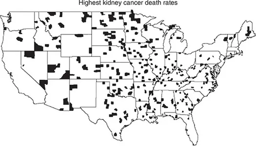
The maps shown in Figure 1.1 depict kidney cancer mortality rates for US counties (Gelman and Nolan, 2017). One map shows the counties that are in the highest decile – that is, they are in the top 10% with respect to kidney cancer mortality rates.

Figure 1.1a Counties in the highest decile for kidney cancer mortality (1980–5)

Source: Gelman and Nolan (2017:14). Reproduced with permission of Oxford University Press.

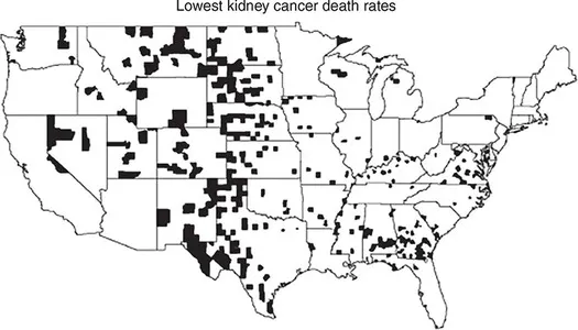
Figure 1.1b Counties in the lowest decile for kidney cancer mortality (1980–9)

Source: Gelman and Nolan (2017:15). Reproduced with permission of Oxford University Press.

The other map shows those counties in the lowest decile – these are the counties that have the country’s lowest kidney cancer mortality rates. The maps have some similar patterning – in both maps, the Midwest and the Great Plains stand out. Some counties in these regions have the country’s highest rates; others have the country’s lowest rates. Thus the region with the lowest rates is the same as the region with the highest – both lowest and highest rates occur in the Midwest and the Great Plains.

Why might this be? The reason has to do with the low denominators used to compute the rates in this part of the country. A mortality rate is based upon the number of deaths, divided by the size of the population at risk of dying. In the Midwest and the Great Plains, population sizes (and hence the denominators of the rates) are relatively low. Just one case of kidney cancer could cause the rate to be high if the population was low enough. Similarly, if the population was very low, it would not be surprising to get an observed rate of zero. In low population counties then, rates are more variable.

A similar effect is observed when tossing coins. If you toss a coin ten times, rates at which the coin turns up heads are more variable than when you toss the coin 1,000 times. It would not be too surprising to get, say, anywhere from three to seven heads if you toss it ten times (i.e., rates of heads between 0.3 and 0.7 would not be surprising). But you certainly wouldn’t expect this much variability if you were to toss the coin 1,000 times (the rate at which the coin came up heads, in repeated experiments, would be across a much narrower range (centered on 0.5) than the range from 0.3 to 0.7).

Simply stated, small samples display more variability than large samples. And we see that this has consequences for map reading. We need to be careful when we interpret maps of rates, because the places with the highest (and lowest) rates may have those rates not because their inherent risk is high (or low), but simply because they have small denominators.

1.3 Some Motivating Problems

1.3.1 Perceptions of Randomness – Visual Assessment of Maps

Part A

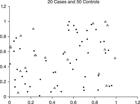
Figure 1.2 is a map of the locations of 20 cases of disease and the locations of 50 healthy controls. Suppose that you are a health analyst for a local agency and you are asked to find any region or regions that have more cases than would be expected, relative to the distribution of controls. Take the map (or a copy of it!) in Figure 1.2 and circle these regions.

Figure 1.2 20 cases and 50 controls

Part B

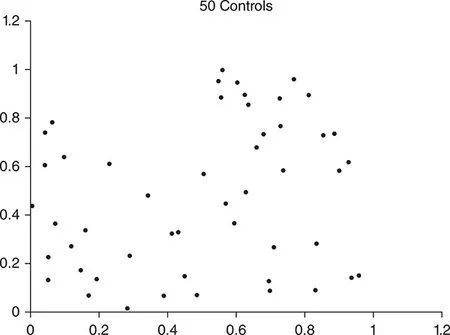
The map in Figure 1.3 contains the locations of 50 healthy individuals drawn at random from a hypothetical population. This hypothetical population is randomly distributed throughout the region. Suppose that there are 20 individuals in the population who have a particular disease. Furthermore, we will assume that the disease risk is spatially uniform – there are no locations on the map that have a raised or suppressed risk of disease.

Figure 1.3 50 controls

Your task in this exercise is to place 20 points on the map, each representing the location of an individual with the disease. As you do so, keep in mind that the spatial distribution of the 20 points should not be influenced by the locations of the 50 healthy individuals (since the population is distributed randomly, and disease risk is spatially random). Thus the geographic distribution of cases should not be clustered or dispersed, relative to the distribution of healthy controls.

Discussion

The map in Part A was generated by choosing both the case and control locations at random. There is in fact no clustering of cases relative to controls, and thus nothing should have been circled. Of course a few cases may be near to one another just by chance. The human eye is good at organizing spatial information and “seeing” what it thinks are significant geographic clusters of points; the eye is not as good at distinguishing whether points that are close together could have arisen by chance alone.

For the exercise in Part B, look at the nearest point for each of the 20 cases on the map. In some instances the nearest point will be a case and in other instances it will be a control. Do this for each case, and tabulate the number of times that the nearest point is a case. For maps where cases are randomly located with respect to controls, the expected number of such case–case pairs is 20(19/69) = 5.5. To see why this is, recognize that when examining a particular case, there are 19 + 50 = 69 other points on the map, and 19 of them are cases. Thus the probability that a point chosen randomly from these other points is a case is equal to 19/69. Since we repeat this 20 times (once for each case), the expected number of case–case pairs is 20(19/69) = 5.5.

Observing anything more than 5.5 case–case pairs indicates a tendency for cases to cluster near one another. If the number of case–case pairs is less than 5.5, this indicates a tendency for cases to be closer to controls than would be expected by chance alone. There is a tendency for individuals to choose case locations that are not near other case locations; hence the number of case–case pairs on maps created by individuals is often less than that expected in a random pattern. This underscores the ineffectiveness of people at assessing spatial randomness, and helps to motivate the need for spatial statistical methods.

In this particular example, there is another way to assess the spatial pattern of cases. Since the population (and the spatial distribution of controls) is random, the location of cases should also be random. There are 25 cells on the map....