A Beginner's Guide to Structural Equation Modeling

Tiffany A. Whittaker, Randall E. Schumacker

• Publisher: Routledge
• Year: 2022
• ISBN:
  9781000569780
• Edition: 5
• Topic: Psychology
• Subtopic: Research & Methodology in Psychology
• Index: Psychology

A Beginner's Guide to Structural Equation Modeling, fifth edition, has been redesigned with consideration of a true beginner in structural equation modeling (SEM) in mind. The book covers introductory through intermediate topics in SEM in more detail than in any previous edition.

All of the chapters that introduce models in SEM have been expanded to include easy-to-follow, step-by-step guidelines that readers can use when conducting their own SEM analyses. These chapters also include examples of tables to include in results sections that readers may use as templates when writing up the findings from their SEM analyses. The models that are illustrated in the text will allow SEM beginners to conduct, interpret, and write up analyses for observed variable path models to full structural models, up to testing higher order models as well as multiple group modeling techniques. Updated information about methodological research in relevant areas will help students and researchers be more informed readers of SEM research. The checklist of SEM considerations when conducting and reporting SEM analyses is a collective set of requirements that will help improve the rigor of SEM analyses.

This book is intended for true beginners in SEM and is designed for introductory graduate courses in SEM taught in psychology, education, business, and the social and healthcare sciences. This book also appeals to researchers and faculty in various disciplines. Prerequisites include correlation and regression methods.

Chapter 1Introduction

DOI: 10.4324/9781003044017-1

What is Structural Equation Modeling?

Structural equation modeling (SEM) depicts relations among observed and latent variables in various types of theoretical models, providing quantitative tests of hypotheses by the researcher. Basically, various theoretical models may be hypothesized and tested with SEM. The SEM models hypothesize how sets of observed variables are interrelated, how sets of variables define constructs, and/or how different constructs are related to each other. For example, an educational researcher might hypothesize that a student’s home environment influences their subsequent achievement in school. A marketing researcher may hypothesize that consumer trust in a corporation leads to increased financial performance for that corporation. A health care professional might believe that increased stress levels can result in increased health risks.

In each example, based on theory and empirical research, the researcher wants to test whether a set of observed variables are related or define the constructs that are hypothesized to be related in a certain way. The goal of SEM is to test whether the theoretical model is supported by sample data. If the sample data support the theoretical model, then the hypothesized relations among the constructs are strengthened. If the sample data do not support the theoretical model, then an alternative theoretical model may need to be specified and tested. Consequently, SEM allows researchers to test theoretical models in order to advance our understanding of the complex relations among constructs.

SEM can test various types of theoretical models. The first types discussed in this book include linear regression, path, and confirmatory factor analysis (CFA) models, which form the basis for understanding the many different types of SEM models. The regression models use observed variables, while path models can use either observed or latent variables. CFA models, by definition, use observed variables to define latent variables. Thus, these two types of variables, observed variables and latent variables, are used depending upon the type of SEM model.

Notation and Terminology

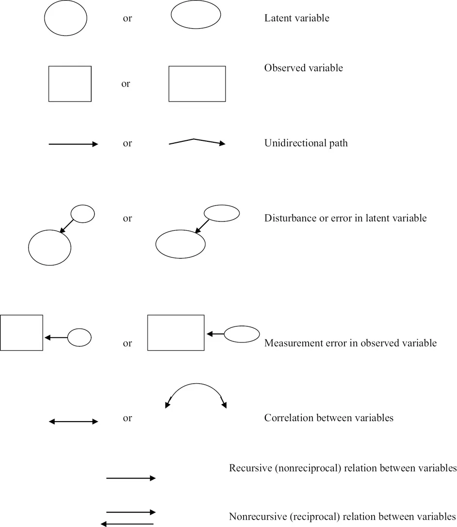
Structural equation models are commonly demonstrated in diagrams with various symbols representing observed and latent variables and their interrelationships, such as squares, circles, one-headed arrows, and two-headed arrows. Figure 1.1 includes a summary of the common diagrams used in SEM. In SEM diagrams, squares symbolize observed variables whereas circles symbolize unobserved or latent variables.

Figure 1.1:Common SEM diagram symbols

Latent variables, also called constructs or factors, are variables that are not directly observed or measured. Latent variables are not directly observed or measured, but are inferred from a set of observed variables that we actually measure using tests, surveys, scales, and so on. For example, intelligence is a latent variable that represents a psychological construct. The confidence of consumers in American business is another latent variable, one representing an economic construct. Stress is a third latent variable, one representing a health-related construct.

The observed variables, also called measured, manifest, or indicator variables, are a set of variables that we use to define or infer the latent variable or construct. Researchers use several indicator variables to define a latent variable. For example, the Wechsler Intelligence Scale for Children-Revised (WISC-R) is an instrument that produces several measured composite variables (or observed scores), which are used to infer different components of the construct of a child’s intelligence. These variables could be used as indicator variables of intelligence to indicate or define the construct of intelligence (a latent variable). The Dow Jones index is a standard measure of the American corporate economy strength construct. Other indicator variables that could be used in addition to the Dow Jones index to define economy strength (a latent variable) include gross national product, retail sales, and export sales. The number of times a person exercises per week is an indicator of a health-related latent variable that could be defined as Health Risk. Other indicator variables that could also be used as an indicator for this Health Risk factor include diet and body mass index (BMI). These models are commonly referred to as confirmatory factor analysis (CFA) or measurement models, which test whether the relationships among indicator variables are explained well by the latent variable. These measurement models can then be used in larger structural models which test the hypothesized relations among the latent variables.

Observed and latent variables are defined as either independent variables or dependent variables. An independent variable, also referred to as an exogenous variable, is a variable that is not influenced or directly affected by any other variable in the model. A dependent variable, also called an endogenous variable, is a variable that is influenced or directly affected by other variables in the model. Figure 1.1 illustrates other symbols used in SEM. One-headed arrows represent direct effects while two-headed arrows represent that two variables are simply related. The researcher specifies the independent (exogenous) and dependent (endogenous) variables and other interrelationships in a model using one-headed and two-headed arrows.

For instance, the educational researcher hypothesizes that a student’s home environment (independent/exogenous latent variable) influences school achievement (dependent/endogenous latent variable). The marketing researcher believes that consumer trust in a corporation (independent/exogenous latent variable) leads to increased financial performance for that corporation (dependent/endogenous latent variable). The health care professional wants to determine whether stress (independent/exogenous latent variable) influences health risk (dependent/endogenous latent variable).

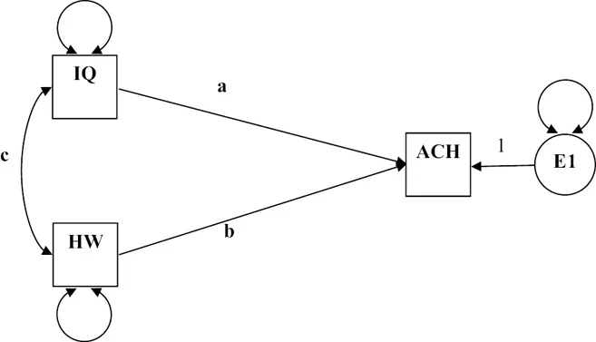
The basic SEM models (regression, path, and CFA) illustrate the use of observed variables and latent variables which are defined as independent or dependent in the model. A regression model consists solely of observed variables where a single observed dependent variable is predicted or explained by one or more observed independent variables. For example, a child’s intelligence and their time spent on homework (observed independent variables) are used to predict the child’s achievement score (observed dependent variable). A depiction of this model is shown in Figure 1.2, wherein the intelligence (IQ) variable and the homework time (HW) variable are hypothesized to directly impact achievement (ACH) while covarying. You will notice that variances (represented by a circular two-headed arrow) are associated with both IQ and HW because they are independent (exogenous) variables. This is because these variables are free to vary with freely estimated variances given that they are not directly impacted by other variables in the model. You will also notice that an error variance is associated with ACH because it is a dependent (endogenous) variable. Unless both IQ and HW explain 100% of the variance in ACH, there will be unexplained variability in ACH that is not explained by both IQ and HW. Thus, dependent (endogenous) variables in SEM have error terms associated with them. These are typically represented via circles in diagrams because they are also unobserved or latent variables. They also have direct effects on their respective dependent (endogenous) variables. Thus, errors are usually considered independent (exogenous) variables because they have direct effects on dependent (endogenous) variables. As such, errors also have variances (represented by a circular two-headed arrow) associated with them.

Figure 1.2:Achievement multiple regression model

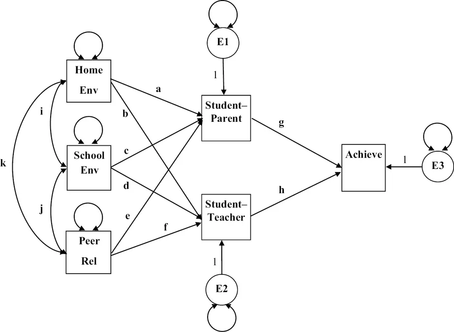
A path model can also be specified entirely with observed variables, but the flexibility allows for multiple observed independent variables and multiple observed dependent variables – for example, export sales, gross national product, and NASDAQ index (observed independent/exogenous variables) influence consumer trust and consumer spending (observed dependent/endogenous variables). Path models are generally more complex models than regression models, include direct and indirect effects, and can include latent variables. Illustrated in Figure 1.3 is an observed variable path model wherein home environment, school environment, and relations with peers (covarying independent/exogenous variables) explain student–parent relations and student–teacher relations (dependent/endogenous variables), which subsequently directly impact student achievement (dependent/endogenous variable).

Figure 1.3:Achievement observed variable path model

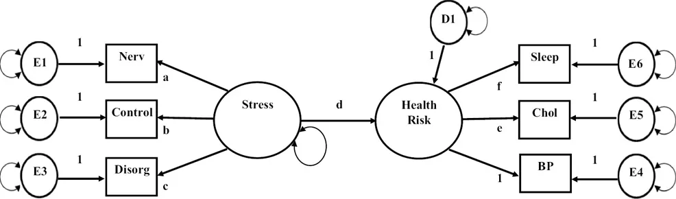
Confirmatory factor models consist of observed variables that are hypothesized to measure both independent and dependent latent variables. Figure 1.4 illustrates an SEM model wherein one factor directly impacts another factor. As shown in Figure 1.4, responses to items asking how often participants have felt nervous, felt not in control of life events, and felt disorganized in the last week are observed measures of the independent (exogenous) latent variable, Stress, while blood pressure, cholesterol, and restless sleep are observed measures of the dependent (endogenous) latent variable, Health Risk. The dependent (endogenous) Health Risk factor has error associated with it, representing unexplained variability. You will notice in Figure 1.4 that the indicator variables are dependent (endogenous) variables in measurement models with errors (E1–E6). Errors associated with latent dependent (endogenous) factors are commonly differentiated from the errors associated with observed dependent (endogenous) variables and typically called disturbances (e.g., D1; see Figure 1.4).

Figure 1.4:Stress and health risk SEM model

History of Structural Equation Modeling

To discuss the history of structural equation modeling, we explain the following four types of related models and their chronological order of development: regression, path, confirmatory factor, and structural equation modeling (see Matsueda, 2012 for additional coverage of the history of SEM). The first models involve linear regression models which use a correlation coefficient and the least squares criterion to compute regression weights. Regression models were made possible because Karl Pearson created a formula for the correlation coefficient in 1896 that provided an index for the relation between two variables (Pearson, 1938). The regression model permits the prediction of observed dependent variable scores (Y scores), given a linear weighting of a set of observed independent scores (X scores). The linear weighting of the independent variables is done using regression coefficients, which are determined based on minimizing the sum of squared residual error values. The selection of the regression weights is therefore based on the Least Squares Criter...