Financial Engineering with Copulas Explained

J. Mai, M. Scherer

• Publisher: Palgrave Macmillan
• Year: 2014
• Print ISBN: 9781137346308
• eBook ISBN: 9781137346315
• Topic: Business
• Subtopic: Financial Engineering
• Index: Business

This is a succinct guide to the application and modelling of dependence models or copulas in the financial markets. First applied to credit risk modelling, copulas are now widely used across a range of derivatives transactions, asset pricing techniques and risk models and are a core part of the financial engineer's toolkit.

1	What Are Copulas?

This chapter introduces a concept for describing the dependence structure between random variables with arbitrary marginal distribution functions. The main idea is to describe the probability distribution of a d-dimensional random vector by two separate objects: (i) the set of univariate probability distributions for all d components, the so-called ‘marginals’, and (ii) a ‘copula’, which is a d-variate function that contains the information about the dependence structure between the components. Although such a separation into marginals and a copula (if done carelessly) bears some potential for irritations (see Section 7.2 and [Mikosch (2006)]), it can be quite convenient in many applications. The rest of this chapter is organized as follows. Section 1.1 presents two examples which motivate the necessity for the use of a copula concept. Section 1.2 presents Sklar’s Theorem, which can be seen as the ‘fundamental theorem of copula theory’.

1.1 Two Motivating Examples

The following examples illustrate situations where it is convenient to separate univariate marginal distributions and dependence structure, which is precisely what the concept of a copula does.

1.1.1 Example 1: Analyzing Dependence between Asset Movements

We consider three time series with daily observations, ranging from April 2008 to May 2013: the stock price of BMW AG, the stock price of Daimler AG, and a Gold Index. Intuitively, we would expect the movements of Daimler and BMW to be highly dependent, whereas the returns of BMW and the Gold Index are expected to be much more weakly associated, if not independent. But how can we measure or visualize this dependence? To tackle this question, we introduce a little bit of probability theory by viewing the observed time series as realizations of certain stochastic processes. For the sake of notational convenience, we abbreviate to B = BMW, D = Daimler, and G = Gold. First, each individual time series

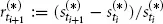
, for * ∈ {B, D, G}, is transformed to a return time series

via

, i = 0, 1, 2, . . . , n – 1. Next, we assume that the returns are realizations of independent and identically distributed (iid) random variables.¹ More precisely, the vectors

, i = 1, . . . , n, are iid realizations of the random vector (R^(B) , R^(D) , R^(G)). We want to analyze the dependence structure between the components of this random vector. Under these assumptions, the dependence between the movements of the BMW stock, the Daimler stock, and the Gold Index are completely described by the dependence between the random variables R^(B), R^(D), and R^(G). For the mathematical description of this dependence there exists a rigorous theory, part of which is introduced in this book. We now provide a couple of intuitive ideas of what to do with our data.

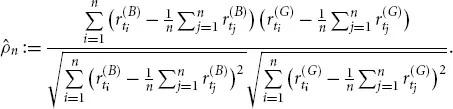
(a)Linear correlation: The notion of a ‘correlation coefficient’ is the kind of dependence measurement that is omnipresent in the literature as well as in daily practice. Given the two time series of BMW and Gold Index returns, their empirical (or historical) correlation coefficient is computed via the formula

Intuitively speaking, this is the empirical covariance divided by the empirical standard deviations. This number is known to lie between – 1 and +1, which are interpreted as the boundary values of a scale measuring the strength of dependence. The value – 1 is understood as negative dependence, the middle value 0 as uncorrelated, and the value +1 as positive dependence. Statistically speaking, the number

, which is computed only from observed data, is an estimate for the theoretical quantity

Generally speaking, the correlation coefficient ρ is one dependence measure (among many), and it is by far the most popular one. However, it has its shortcomings (see Chapter 3). Copula theory can help to overcome these limitations, because it provides a solid ground to axiomatically define dependence measures.

(b)Scatter plot: One of the most obvious approaches to visualize the dependence between the return variables, say R^(B) and R^(G), is to plot the observed historical data into a two-dimensional coordinate system, which is done in Figure 1.1. Such an illustration is called a ‘scatter plot’. In the same figure the scatter plots for the observed values of R^(B) vs. R^(D) and R^(D) vs. R^(G) are also provided in order to judge on the qualitative differences between the dependence structures. All scatter plots appear to be centered roughly around (0, 0); only the two automobile firms exhibit a scatter plot which is m...

Table of contents

• Cover
• Title
• 1 What Are Copulas?
• 2 Which Rules for Handling Copulas Do I Need?
• 3 How to Measure Dependence?
• 4 What are Popular Families of Copulas?
• 5 How to Simulate Multivariate Distributions?
• 6 How to Estimate Parameters of a Multivariate Model?
• 7 How to Deal with Uncertainty Concerning Dependence?
• 8 How to Construct a Portfolio-Default Model?
• References
• Index