Optimization Methods for Gas and Power Markets

Theory and Cases

Enrico Edoli,Stefano Fiorenzani,Tiziano Vargiolu

• Publisher: Palgrave Macmillan
• Year: 2016
• ISBN:
  9781137412973
• Topic: Volkswirtschaftslehre
• Subtopic: Ökonometrie

As power and gas markets are becoming more and more mature and globally competitive, the importance of reaching maximum potential economic efficiency is fundamental in all the sectors of the value chain, from investments selection to asset optimization, trading and sales. Optimization techniques can be used in many different fields of the energy industry, in order to reduce production and financial costs, increase sales revenues and mitigate all kinds of risks potentially affecting the economic margin. For this reason the industry has now focused its attention on the general concept of optimization and to the different techniques (mainly mathematical techniques) to reach it. Optimization Methods for Gas and Power Markets presents both theoretical elements and practical examples for solving energy optimization issues in gas and power markets. Starting with the theoretical framework and the basic business and economics of power and gas optimization, it quickly moves on to review the mathematical optimization problems inherent to the industry, and their solutions – all supported with examples from the energy sector. Coverage ranges from very long-term (and capital intensive) optimization problems such as investment valuation/diversification to asset (gas and power) optimization/hedging problems, and pure trading decisions.This book first presents the readers with various examples of optimization problems arising in power and gas markets, then deals withgeneral optimization problems and describes the mathematical tools useful for their solution. The remainder of the book is dedicated to presenting a number of key business cases which apply the proposed techniques to concrete market problems. Topics include static asset optimization, real option evaluation, dynamic optimization of structured products like swing, virtual storage or virtual power plant contracts and optimal trading in intra-day power markets. As the book progresses, so too does the level of mathematical complexity, providing readers with an appreciation of the growing sophistication of even common problems in current market practice. Optimization Methods for Gas and Power Markets provides a valuable quantitative guide to the technicalities of optimization methodologies in gas and power markets; it is essential reading for practitioners in the energy industry and financial sector who work in trading, quantitative analysis and energy risk modeling.

1

Optimization in Energy Markets

1.1 Classification of optimization problems

In the Preface, we mentioned that optimization problems represent a class of mathematical problems that we cannot consider always homogeneous. Different kinds of problems ask for different representation and solution tools. Hence, a bit of classification may be worthwhile for the sake of clarity.

1.1.1 Linear versus nonlinear problems

The distinction between linear and nonlinear optimization problems has to do with the shape of the objective function and functional constraints. If both constraints and objective functions are linear, we can (obviously) talk about linear optimization problems, while in all the other situations we will have a nonlinear optimization problem.

Linearity strongly impacts on the solution methods we can apply to the problem: for the solution of linear optimization problems, fast solution algorithms, able to reach exactly the optimal solution of the problem, are often available, while in all the other cases we do not have the guarantee of such a simple and fast solution method.

Most of the time, the linear representation of a problem is a helpful simplification we impose on the problem itself in order to make it simpler to solve. Mathematicians often refer to “the art of linearization” in order to make explicit the fact that making linear a nonlinear problem is an almost esoteric exercise which requires experience and full knowledge of the true problem. We need to carefully understand whether linearization is possible or not and assess the kind of problems simplifying assumptions are carrying on for our specific problem. Nevertheless, when allowed and not distortive, linearization is extremely helpful, especially when our focus is the practical determination of an effective solution (even if not the best one) to our problem and not the formal representation and study of the problem itself.

1.1.2 Deterministic versus stochastic problems

We are not always able to measure or observe the current value of many parameters affecting our target function, mainly because most of the optimization problems we are interested in deal with quantities that are unknown at the time when the optimization is performed, such as the future profit and loss of a financial instrument. Typically, in those cases we are only able to make some assumptions on the unknown parameters or to speculate about their future behavior, but are not able to know the exact value of them. In such cases, we often make probabilistic assumptions on those parameters, based on statistical observations. We say that such optimization problems have a stochastic nature. In more practical terms, also our decisions need to be taken under uncertainty. On the other hand, if we are completely able to measure all the variables that have a direct impact on our optimization problem, the problem is called deterministic.

Real-life decisions are rarely taken under a fully complete information set, i.e., an information set without uncertainty about relevant factors which affect decisions. Most of the time, we are interested in optimizing our behavior with respect to future events that, by definition, are unknown at the current state. Moreover, even when we aim at adjusting our decisions with respect to intrinsically deterministic factors, we are always affected by measurement errors which induce uncertainty (small or big) on the final outcome. As stated for linearization, framing a problem as a deterministic problem is most of the time a kind of simplification made up by the decision-maker, rather than a real case. Deterministic problems are always easier and faster to solve than stochastic ones, but when this simplification is introduced, we need to take into account that we are dealing with an approximation of the true (and more complex) solution.

1.1.3 Static versus dynamic problems

The concepts of static and dynamic relate directly with that of motion through time but, when we consider optimization problems, not all those that have a time dimension must be considered as dynamic problems.

We define an optimization problem as dynamic only when it requires decisions to be taken through time, and the sequence of optimal decisions are not independent of each other. In other terms, a dynamic optimization problem is when decisions or actions taken at a certain moment can potentially affect those we could take in subsequent moments.

On the other hand, a static optimization problem is a problem where the sequence of decisions, even if spread through a certain time frame, are temporally independent. In a static problem we will select the current optimal choice without considering the impact it may have on future choices, or better we will not consider co-dependency because we assume decisions are independent of each other.

The reader should note that considering the natural dynamicity and co-dependency of a certain optimization problem is not equivalent to the repetition several times of a static exercise through time. Considering the natural co-dependency that many optimization problems have is really a complex task. It is often complex to represent realistically the decisions sequence (framing the optimization problem), and even more complex to solve it somehow.

In real life, we are almost always asked to take decisions whose effects will perpetuate in the future (short-term future to long-term future), and each action we engage in will modify peremptorily the set of our future choices, opening some opportunities and closing some others. Decisions in business, and in energy markets in particular, do not differ. Hence, many of the problems we will face while searching for the best result will be most of the time complex (nonlinear), surrounded by uncertainty (stochastic) and extremely dynamic. Basically, we are always in the worst situation! However, not in all the situations where we are asked to take a business decision do we need the maximum potential accuracy. In some situations we just need an indication, while in some other situations a precise decision support is necessary.

Typically, the longer the time horizon in which to observe the effects of our business decision, the more we are inclined to simplify the optimization problem we are facing, ignoring also the impacts that associated decisions will have on other problems of shorter-term horizon. This sounds really like a paradox, because it implies that the more the problem is important for our business, the more we base our decisions on human emotions instead of adopting more formal approaches. On the other hand, it is true that the longer the time horizon of the problem, the higher the complexity of the decisions and the uncertainty which affects relevant variables. Hence, for those problems, a formal framing and solving of the true problem would be impractical and simplifications are necessary in order to derive at least an indication of what is best to do.

In the remaining part of the chapter we will propose some examples of business optimization problems which are typical of modern power and gas sectors. These problems will span from investment decisions to trading strategies, with the scope of correctly orienting the reader towards the correct framing of different classes of optimization problems, and leaving the solution methods for the subsequent chapters.

1.2 Optimal portfolio selection among different investment alternatives

In modern financial theory, portfolio selection is historically associated with the seminal work of Markowitz (1952). Markowitz’s problem can be summarized in the following way: an investor can allocate its capital into N assets and must decide (in advance with respect to the investment operation) how much to invest in each single asset, trying to balance the expected return and the risk of the portfolio. Markowitz’s problem deals with financial assets; hence, these are infinitely divisible assets that can be liquidated at any time in the market. An asset’s return is basically the proportional increment of value that the asset faces during the holding period. The portfolio’s risk is univocally measured by the variance of its return.

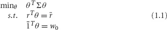
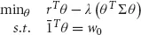
Markowitz’s problem is a single period static optimization problem that can be formalized as follows

where

is the expected return of the assets,

is the variance-covariance matrix among the assets, and

are the amounts invested in every asset. The expected return of the portfolio is given by r^Tθ and the variance of the portfolio by θ^T Σθ, that is the quantity we want to minimize given a fixed rate of return

; the total amount invested in each single asset must add up to the initial amount w₀.

Sometimes, the risk-minimizing approach of the classical Markowitz’s problem is replaced by a more practical risk-adjusted performance maximization of the following type

without substantial changes to the nature of the optimization problem.

When our ...