The Political Economy of India's Growth Episodes

Sabyasachi Kar,Kunal Sen

• Publisher: Palgrave Pivot
• Year: 2016
• ISBN:
  9781352000269
• Topic: Politik & Internationale Beziehungen
• Subtopic: Handel & Tarife

'This book is different from most other attempts to understand the politics of Indian economic development. Breaking down the last 65+ years of Indian development into several episodes of growth, it provides a rich set of insights into the political economy of the Indian development process and is a valuable addition to the literature.' –Pranab Bardham, University of California, Berkeley, USA

'Sustained economic growth in the world's largest democracy is critically important to human well-being, but the ups and downs of growth in India are not well-understood. This book provides a fresh and insightful approach to understanding what drives the starts of booms and the onset of slowdowns.' –Lant Pritchett, Harvard University, USA

'This is a little book with big arguments. The authors' explanation of the changing character of the deals done between political and business elites makes for the most original contribution to studies of the political economy of Indiandevelopment since Pranab Bardhan's seminal work of the early 1980s' –John Harriss, Simon Fraser University, Vancouver, Canada

This book moves beyond the usual economic analysis of the Indian growth story and provides a fresh perspective on the determinants of growth episodes in post-independence India, based on its political economy. Using a robust and novel technique, the authors identify four such episodes during this period. The first, running from the 1950s to 1992, was mostly characterized by economic stagnation, with a nascent recovery in the eighties. The second, covering the period 1993 to 2001, witnessed the first growth acceleration in the economy. A second acceleration ran from 2002 to 2010. The fourth and final episode started with the slowdown in 2010 and continues to this day. The book provides a theoretical framework that focuses on rent-structures, institutions and the polity, and demonstrates how changes in these can explain the four growth episodes. Kar and Sen argue that the transitions from one growth episode to another can be explained by the bi-directional relationship between growth outcomes and institutional arrangements, and by the manner in which institutional arrangements and their transitions are determined by the political bargains struck between the elite groups in Indian society.

© The Author(s) 2016

Sabyasachi Kar and Kunal SenThe Political Economy of India's Growth EpisodesBuilding a Sustainable Political Economy: SPERI Research & Policy10.1057/978-1-352-00026-9_1

Begin Abstract

1. A Political Economy Reading of India’s Growth Experience

Sabyasachi Kar¹ and Kunal Sen²

(1)

Institute of Economic Growth, University of Delhi, Delhi, India

(2)

University of Manchester, Manchester, Lancashire, UK

Abstract

The introductory chapter starts by highlighting the principal theme of the book, that is, the relationship between political economy factors and growth episodes in India. It goes on to provide the nuts and bolts of this analysis—defining growth episodes, discussing earlier studies that have identified growth episodes in India and pointing out the weaknesses in these approaches. Presenting an alternative and more robust framework for identifying episodes, the chapter identifies three complete and one ongoing growth episode for the Indian economy. Next, it contextualizes the study by discussing influential contributions that have analysed the political economy of growth in India in the past. Finally, it traces important political economy trends over the post-independence period, providing a base for their introduction in subsequent chapters.

Keywords

Growth episodesIndiaInstitutional spacePolitical space

End Abstract

Introduction

For decades following its independence from colonial rule, the Indian economy suffered from poor growth outcomes which famously came to be described as “the Hindu rate” of growth. Sometime during the late seventies or early eighties, things started to change for the better and by the second half of the 1990s and 2000s, there was a complete turnaround with India joining the small group of countries that were growth success stories. Recently, this narrative of India’s emerging growth miracle came to be questioned when growth rates slowed down considerably after 2010. However, a nascent recovery in the last few years, combined with China’s clear slowdown, has now made India the strongest contender for the fastest growing “emerging economy” in the world currently.

The factors underlying high growth in India have been analysed by a number of influential studies and two alternative views have evolved on this issue. The first view is that the policy regime—which was markedly pro-socialist, pro-poor and somewhat anti-business during the sixties and seventies—turned pro-business by the early eighties (Rodrik and Subramaniam 2004; Kohli 2006). This change was manifested mostly in terms of the preferential treatments and incentives that established business houses received from the government rather than significant changes in the economic laws to bring about more competition. According to the proponents of this view, this change in approach—which started sometime during the eighties—significantly bettered the property rights environment, leading to higher investment and growth. The second view is that it is the economic reforms in the early nineties (with significant relaxation of some of the draconian laws affecting investments and imports) that led to overall lowering of costs, increased productivity and resulted in higher growth rates in this period (Ahluwalia 2002; Srinivasan and Tendulkar 2003). The two views have something in common—both identify institutional changes as the trigger that led to higher growth rates. The critical difference between the two views is that the first focuses on institutional arrangements where the state deals directly with individual businesses, usually established and large business houses, in order to encourage growth, whereas the second view focuses on the state encouraging the whole range of private sector firms through better institutional (and other infrastructure) facilities.

In our view, the institutional arrangements described in the two views above have both contributed in their own ways towards higher growth in the Indian economy. To that extent, both the views have contributed to the understanding of the Indian growth experience. However, both of these approaches have stopped short of addressing a second and very crucial link in the institutions and growth relationship, which is that growth outcomes also usually have feedback effects on institutional arrangements. In this book, we present a new conceptual framework that shows how the bidirectional feedback effects between growth outcomes and institutional arrangements give rise to growth transitions. Using this framework, we first identify distinct “episodes” of growth for the Indian economy and then analyse the transitions from each of these growth episodes to the next. We also show that these institutional arrangements and their transitions are determined by the political bargains struck between the elite groups in a society. This is the defining characteristic of our “political economy” approach to explaining growth episodes.

As the title suggests, this book attempts to explain India’s growth episodes—particularly the institutional arrangements and political factors that gave rise to them. This introductory chapter will provide the basics—defining growth episodes, discussing the studies that have identified growth episodes in India, pointing out the weaknesses in these approaches and presenting an alternative framework for identifying episodes that are more robust. It will also discuss studies that have analysed the political economy of growth in India as this will provide a background to our book.

A Brief Description of Post-Independence Growth in India

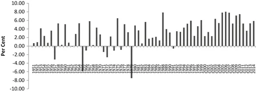
We start with a brief analysis of the Indian growth experience since the fifties. Figure 1.1 shows the annual growth rates of per capita income for this period. It can be seen quite clearly from this figure that there have been significant changes in the nature of growth over time. Till about 1990, we find that growth has been very erratic, with higher growth rates inevitably followed by very low or even negative growth rates. This resulted in average growth rates being quite low in this period. In the post-nineties period, the growth rate became steadier, pulling up average growth rates considerably. Within this period, we can also make out two distinct clusters—one in the nineties and the second between 2000 and 2010. It also seems from the graph that the second cluster gives rise to higher average growth rates compared to the first cluster. As we shall see later on in this chapter, these growth outcomes give rise to three complete growth episodes for the Indian economy.

Fig. 1.1

Annual growth of per capita output (per cent per annum) Source: National Income Accounts, Central Statistical Organisation, various issues, our calculation

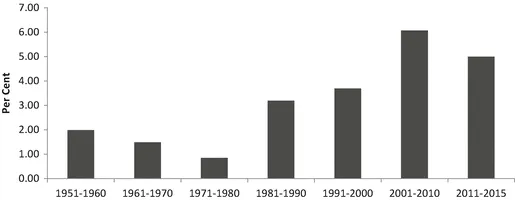
Figure 1.2 depicts the same growth rates as decadal averages. This helps us to understand that the Hindu rate of growth regime was in fact a continuous deterioration of growth outcomes. It also shows that the turnaround has led to a gradual but accelerating period of growth rates, with a little slowing down in the last few years.

Fig. 1.2

Decadal averages of growth of per capita output (per cent per annum) Source: National Income Accounts, Central Statistical Organisation, various issues, our calculations.

It is common to find decadal growth rates like those in Fig. 1.2 being used as growth episodes, that is, as a unit of analysis of medium-term growth behaviour of individual countries (or even in cross country analysis as in, say, Barro and Sala-i-Martin (2003)). Unfortunately, any such approach usually ignores the fact that medium-term growth rates are highly volatile in most countries—particularly developing ones (see Pritchett 2000; Rodrik 1999, 2003; Hausmann et al. 2006; Aizenman and Spiegel 2010) Thus, the decadal average growth rates for these countries may consist of distinct periods of very successful growth and periods of not-so-successful growth—and in some cases—even growth failures (Jones and Olken 2008).

Clearly, using decadal averages as proxies for medium-term growth episodes is misleading as they fail to capture this variability in growth dynamics. In order to understand the genuine “booms and busts” in growth behaviour in these countries, the methodological framework must consist of two parts. The first part must define a methodology to identify all distinct growth episodes for a country. The second part has to then explain the dynamics that leads a country to transition through each of the growth episodes. In order to take care of the volatility of medium-term growth rates, the identification of growth episodes should ensure that each episode has a single underlying medium-term growth rate (with short-run business cycles around this rate). As we shall see in later sections, this implies that growth episodes of a country differ not only in terms of average growth rates, but also in terms of their duration.

The empirical growth literature has grappled with the identification of medium-term growth episodes for some time, and the approach that has emerged as the most popular is the Bai-Perron (2003) (henceforth BP) technique. The BP method identifies statistically significant structural breaks in the growth rate of a country. In order to do this, the BP method first uses an algorithm that searches all possible sets of breaks (up to a maximum number of breaks) and then determines for each number of breaks, the set that produces the maximum goodness of fit. The statistical tests then determine whether the improved fit produced by allowing an additional break is sufficiently large, given what may be expected by chance (Jones and Olken 2008). Starting with a null of no breaks, sequential tests of k versus k + 1 breaks allow one to determine the appropriate number of breaks. Once the technique identifies all the structural breaks in a country’s growth rate, it defines the period between any two consecutive breaks as a growth episode (with the start and end years of available data being treated as the beginning and ending of the first and last episodes).

The BP approach, unfortunately, suffers from what is known in statistics as a low power of the test. This implies that the approach may not be able to identify genuine breaks in growth rates, especially for countries where the series is highly volatile. This is known as the “true negative” problem. In fact, Bai and Perron (2006) carry out some simulation exercises that confirm this problem conclusively. In order to avoid this problem in the BP method, we adopt an alternative approach to identify episodes of economic growth in India. Before discussing that approach, however, it is useful to look at other studies that have attempted to identify growth episodes for the Indian economy.

Indian Growth Episodes

There has been a small but influential set of studies attempting to identify growth transitions and growth episodes for the Indian economy. Some of these studies have used what could be described as an “eyeballing approach” while others have used more rigorous statistical techniques. Studies belonging to the first group include DeLong (2003) that identifies a break in 1985 and Sen (2007) that identifies the break in the mid-seventies. The second group includes Balakrishnan and Parameswaran (2007), who test for multiple structural breaks on Indian output data using the methodology pioneered by Bai and Perron (1998) described above. Balakrishnan and Parameswaran find a single shift in the GDP series which occurred in 1978–1979 and conclude that India’s growth acceleration occurred from this year onwards. A similar exercise using the BP method is reported by Rodrik and Subramanian (2004) and they also get a growth break in 1979. What do these studies tell us about growth episodes in the Indian economy? Based on data till the early 2000s, all of them indicate that the Indian economy had two episodes of growth—the Hindu rate of stagnation and a subsequent growth acceleration. However, the date of the transition from the lower growth episode to the higher growth episode varies somewhat between these studies.

The approaches used in the studies described above have significant weaknesses. An eyeballing approach is always biased by the researcher’s prior beliefs. The BP method is more rigorous and avoids any prior bias. However, as discussed earlier, it suffers from poor power of the test, making it susceptible to rejecting even genuine breaks. In order to avoid these weaknesses, we follow our own procedure set out in Kar et al. (2013b) where it was used for a large number of countries. Our methodology—like the BP method—is a two-stage procedure for identifying structural breaks in economic growth, where the first stage is identical to the first part of the Bai-Perron (BP, 1998) procedure that involves maximizing the F-statistic to identify candidate years for structural breaks in growth, and the second stage imposes thresholds on the magnitude of the shift in candidate breaks in order to determine the actual breaks (see Kar et al. 2013). Thus, this procedure involves the best fit of the BP method to the data in the first stage and the application of a filter to the breaks identified from the first stage to the second stage. It may be noted that by using filters in the second stage instead of statistical inference (which really leads to the low power in the BP tests), our methodology is able to identify many more “true” breaks compared to the pure statistical approach.

The threshold rules are that the absolute value of the change in the growth rate after a potential break had to be (a) 2 percentage points if it was the first break, (b) 3 percentage points if the potential break was of the opposite sign of the previous break (an acceleration that followed a deceleration or a deceleration that followed an acceleration) and (c) 1 percentage point if the potential break was of the same sign as the previous break (an acceleration that directly followed an acceleration or a deceleration that followed a previous deceleration). Thus, the magnitude filters used in our methodology are also able to take into account the previous history of breaks in any country. To estimate potential breaks, we assumed that a “growth regime” lasts a minimum of eight years (as in Berg et al. (2012)). The use of shorter periods (e.g. three or five years) risks conflation with “business cycle fluctuations” or truly “short run” shocks (e.g. droughts). Longer periods (e.g. 10 or 12 years) reduce the number of potential breaks. Application of this procedure to the PWT7.1 data for 125 countries (eliminating all countries with very small populations and those that did not have long enough data series) for the period 1950–2010 identified 314 structural breaks in growth, with some countries having no breaks (e.g. USA, France, Australia) and others having four breaks (e.g. Argentina, Zambia).

Using this methodology on the Indian data, our procedure identifies the first growth break in 1993 and a second growth break in 2002. It may be noted that there were other candidate breaks including 1985 (which would be consistent with the previous literature on growth breaks in India), but they were not significant enough to be identified as actual breaks by our methodology (nor by the BP methodology with the updated dataset). As in the BP approach, we define the period between any two consecutive breaks as a growth episode with the start and end years of available data being treated as the beginning and ending of the first and last episodes. Thus, based on data from 1950 to 2010 and the growth breaks mentioned above, we identify three growth episodes for India which cover the period 1950 to 1992, 1993 to 2001 and 2002 to 2010, respectively. This is also consistent with our eyeballing of Fig. 1.2 discussed earlier.

As is well-documented by now, the Indian economy lost it...