Managing Commodity Price Risk

George A. Zsidisin, Janet L. Hartley, Barbara Gaudenzi, Lutz Kaufmann

• Publisher: Business Expert Press
• Year: 2016
• Print ISBN: 9781631570636
• eBook ISBN: 9781631570643
• Topic: Business
• Subtopic: Operations
• Index: Business

Almost every organization is exposed to financial risk stemming from commodity price volatility. Risk exposure may be direct, from the prices paid for raw materials transformed into products sold to customers, or indirect, from higher energy, transportation costs, and supplier commodity purchases. Managing Commodity Price Risk: A Supply Chain Perspective provides a range of approaches organizations can implement and adapt for assessing, forecasting, and managing commodity price volatility and reducing financial risk exposure associated with purchased goods and services. Understanding and managing commodity price risk is important for organizations and supply chain professionals due to the significant direct financial effects price volatility has on profitability, organizational cash flow, the ability to competitively price products, new product design, buyer–supplier relationships, and the negotiation process.

SECTION II

Forecasting Commodity Prices

CHAPTER 3

Forecasting Short-Term Commodity Prices

Short- and long-term commodity price forecasts help you to make better risk management decisions. Long-term forecasts are looking out in the future, one year or more. Short-term forecasts look ahead to the next few weeks, months, or quarters.

In this chapter, we describe how to use technical analysis to develop short-term forecasts, and in Chapter 4, we discuss long-term forecasts. Technical analysis reviews historical price patterns, and forecasts are based on assumptions about future price patterns. The only data used in technical analysis are historical prices. The theory supporting technical analysis suggests all marketplace information about a commodity is incorporated into its price. As soon as new information is available about a commodity, the market adjusts to determine a new price. This underlying premise is attributed to Charles Dow,¹ who observed price patterns in the stock market. Dow suggested prices reflect factual information, as well as the expectations and beliefs of all market participants. Therefore, in a technical analysis there is no need for understanding the underlying factors affecting price dynamics; the analysis only uses the price’s historical patterns.

Long-term forecasting uses an approach called fundamental analysis, which we discuss in Chapter 4. Fundamental analysis assumes the relationship between supply and demand drives commodity prices. Fundamental analysis involves examining the underlying forces affecting supply and demand, estimating how supply and demand will change, and then assessing what impact the change might have on price.

Managers use short-term forecasts to make tactical decisions to execute supply chain strategies. How are short-term price forecasts used in the company? For example, based on a price forecast, adjustments can be made on how much and when to buy a commodity. If a commodity’s price is expected to increase, it can be acquired sooner than planned, and if prices are forecast to decrease, can be purchased at a later time. The time frame of these decisions determines the time period for short-term forecasts. Typically, monthly or weekly prices are used when forecasting near-term commodity prices. In our research, for example, we found in 85 percent of the companies, the forecasting frequency is monthly, and in only one case daily prices are used for the forecast. These choices are also influenced by the fact, for many commodities, it is easy to find monthly prices published by external sources. Quarterly or annual price forecasts are also available, but these are then typically used for long-term timeline forecasts.

With shorter time periods, say daily versus weekly prices, there can be a lot of variation in the forecast. Longer time periods, such as quarters, tend to smooth out price variations. If orders are placed infrequently, and the spend level and volatility are relatively low, quarterly or monthly forecasts may be more appropriate. In case of frequent purchases, high levels of spend, and highly volatile prices, developing weekly price forecasts may be a better choice.

The key steps in a technical analysis are described as follows:

1. Gathering historical commodity price data.
2. Identifying price patterns.
3. Selecting a forecasting model.
4. Developing forecasts for the appropriate price pattern (stable, trends, seasonality).
5. Developing forecasts for price patterns with trends.
6. Developing forecasts for seasonal price patterns.
7. Assessing forecast accuracy.
8. Improving the forecast.
9. Monitoring the forecast.

Gathering Historical Commodity Price Data

The first step in technical analysis is to gather historical commodity spot prices for the most recent two to three years. Spot prices are the actual prices paid in the marketplace during a given time period. Companies may have historical records on the actual prices paid for commodities. If price data are not readily available within the company, public sources or subscription services may be available. For example, gasoline, oil, natural gas, and coal prices are publicly available through the U.S. Energy Information Administration. The U.S. Department of Agriculture Economic Research Service provides price data for a number of agricultural commodities including corn, soybeans, and wheat; and the World Bank provides price data on a large number of commodities. Subscription services can be expensive but provide forecasts and market information as well, so they may be a valuable investment for your company. When using historical data from different sources, it is important to ensure they are consistent in terms of grade of the commodity, unit of measure, and time frame. For example, there are six different major classes of wheat, each with different producing regions, varying uses, and consuming countries.²

Identifying Price Patterns

The next step in a technical analysis is to plot the historical price data and identify patterns. This can be done using a spreadsheet plotting the price data for the most recent two to three years in a line graph in the order of occurrence. This is typically represented as a time-series price chart. The monthly wellhead natural gas prices for 2014 to 2016 from the U.S. Energy Information Administration shown in Table 3.1 are plotted in Figure 3.1 to illustrate a technical analysis.

After the price chart is complete, basic patterns are identified in the historical prices. In the short-term, prices can exhibit four basic patterns: stable, trend, seasonal, and shift. A stable pattern is essentially a horizontal line with little movement up or down. A trend shows upward or downward price movements. Seasonal patterns are repeating patterns occurring over time. For example, gasoline prices in the United States typically increase during the summer vacation season. Seasonal patterns may be caused by actual seasonal changes, such as harvesting for an agricultural commodity or changes in consumer demand. A shift is a step change occurring—for example—after a major disruption to supply or demand.

Table 3.1 Natural gas: Citygate prices (US$/1,000 cubic ft.), January 2014 to March 2016

Month	2014	2015	2016
January	$5.56	$4.48	$3.38
February	$6.41	$4.54	$3.46
March	$6.57	$4.35	$3.45
April	$5.64	$3.93
May	$5.90	$4.24
June	$6.05	$4.43
July	$5.99	$4.65
August	$5.49	$4.58
September	$5.51	$4.54
October	$5.16	$4.00
November	$4.91	$3.68
December	$5.15	$3.76

Source: U.S. Energy Information Administration.³

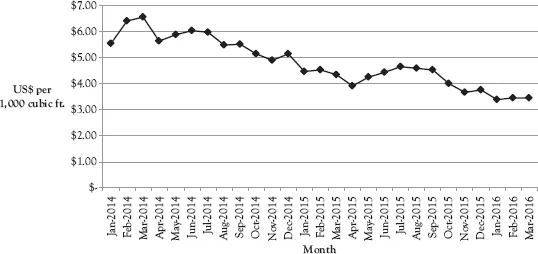
Figure 3.1 Natural gas: Citygate prices, January 2014 to March 2016

Source: U.S. Energy Information Administration.⁴

Besides the basic patterns, some prices may be a combination of patterns. For example, a seasonal pattern can also have an increasing or decreasing trend. In the long-term, a cyclical pattern from economic cycles may also be evident.

Random error is present in all pricing patterns. Over time price patterns change, and for some commodities, frequent changes can occur.

Determining price patterns is more of an art than a science and requires judgment and experience. Since all price patterns contain random error, it is difficult to sort out real changes in patterns from those that are noise. Note the monthly prices for natural gas are shown in Figure 3.1. Overall during this time period there had been a downward trend in price. However, during this period there were some months, for example, April through July 2015 when prices increased. Further, in February and March 2016, prices appear to have stabilized. There is no “right” answer to the patterns, as this depends on judgment, which is gained through experience. So when a trend is occurring, how far will prices increase or decrease? Patterns emerge because of market participants’ beliefs and behaviors. Prices tend to increase or decrease until they hit upper and lower boundaries formed by the behaviors of the market participants. At the upper end is a resistance price that is the “highest” price for the commodity. When an upward trend encounters the resistance price, it typically shifts direction and begins to decline. Similarly, a low price point called support is the price that a decreasing trend typically reverses.

Commodity traders use short-term price charts with frequent intervals, often as short as 1 minute, to identify support and resistant points. For natural gas over the entire time period, as shown in Figure 3.1, the resistance price appears to be $6.57 per 1,000 cubic ft., and the support price is $3.45 per 1,000 cubic ft. The resistance and support prices can change over time. A shift in the pattern caused by a major supply disruption or economic jolt will shift the resistance and support prices.

In technical analysis, there are a number of standard price patterns beyond the scope of this book that experienced analysts use to identify trends and trend reversals. It takes time to study and learn about commodities and begin to develop an understanding of their normal pricing patterns. Understanding pricing patterns provides critical information for making better commodity management decisions.

Selecting a Forecasting Model

Commodity traders use a wide variety of technical analysis tools to understand very short-term pricing patterns, so they can profit from price movements. Supply chain managers, whose objective is to understand commodity price risk and buy to budget, can use a subset of these tools. Some statistical tools useful for short-term forecasting for supply chain management include time-series models, simple linear regression, and seaso...

Table of contents

• Cover
• Title
• Copyright
• Preface
• Acknowledgments
• Section I Background
• Section II Forecasting Commodity Prices
• Section III Managing Commodity Price Risk
• Section IV Cases and Additional Observations
• Notes
• References
• Index
• Adpage