Regression for Economics, Second Edition

Shahdad Naghshpour

• Publisher: Business Expert Press
• Year: 2016
• Print ISBN: 9781631574436
• eBook ISBN: 9781631574443
• Topic: Economics
• Subtopic: Statistics for Business & Economics
• Index: Economics

Regression analysis can be used to establish causal relationships between factors and the response variable. However, in order to be able to do so, economic theory must be used to provide the causal relationship and then regression analysis is applied to verify the validity of the theory. Regression analysis is the most commonly used analytical tool and can be understood without complex mathematics. This book simplifies and demystifies regression analysis. All the examples are from economics and in almost all the cases, real data is used to show the application of the method. By limiting the use of mathematical symbols, the author enables a logical reader to learn regression, without shortchanging the subject. The book is targeted to all business students and executives who need to understand the concept of regression for practical and professional purposes.

CHAPTER 1

The Concept of Regression

Relationship Between Variables

When analyzing phenomena that are affected by other variables, it is necessary to account for contributing factors. Although the association between variables can be complex and of unknown structure, in most cases, it is possible to approximate the relationship using a linear model or models that can be linearized. There are well-established procedures for modeling quantitative and qualitative variables. One such technique is called regression analysis.

In regression analysis, one variable, known as the dependent variable, is explained by one or more variables known as independent, or explanatory, variables. Before presenting a regression model, an examination of a simple model for explaining consumption using income is beneficial. First, however, we need to define the economic concept of marginal propensity to consume (MPC).

Definition 1.1

The MPC represents the change in consumption for a given change in income.

(1.1)

Conceptually, the MPC is the same as the slope of a line in Euclidian geometry, where a dependent variable is expressed as a constant plus the slope times the independent variable, which is similar to the equation of a line. The equation for a line is

(1.2)

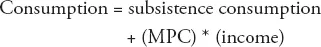
where m is the slope and b is the Y axis intercept. The slope indicates the magnitude of and direction of change in Y due to a one unit change in X. The intercept reflects the value of Y when the line intersects it; the value of X at such point is zero. In Equation 1.1, consumption is the dependent variable (Y) and income is the independent variable (X ). Although the term dependent variable is commonly used in economics literature, other names such as endogenous variable, Y-variable, response variable, or even output are often used as well. Similarly, the term independent variable might be replaced by an explanatory variable, exogenous variable, X-variable, regressor, input, factor, or predictor. The analogy between Equations 1.1 and 1.2 should be evident. MPC is the slope (m) and subsistence consumption is the necessary consumption when income is zero (b), which indicates the intersection point of the consumption line with the income axis.

Equation 1.1 is a good example of the concept of regression, but it is not a regression model. The format for a regression model will be discussed shortly. You are more likely to be familiar with a mathematical than a statistical function such as regression. A mathematical function represents a nonprobabilistic association between a dependent and one or more independent variables; the association is exact and fixed (Figure 1.1 panel A). Such an association is considered to be deterministic, by contrast, a regression model, like all statistical models, is a simplification of reality. It is in fact a claim of a relationship and, thus, a testable hypothesis. The association between the dependent and the independent variable(s) is probabilistic, not deterministic, in that the association is not fixed and involves some element of randomness. It is true on the average only.

Figure 1.1 panel B depicts a probabilistic relationship using pairs of (X, Y) observations relating a dependent variable (Y) to an independent variable (X ). Unlike the points for the equation of a line, the points are scattered around but one can envision a linear pattern as depicted in panel B. The “line” in panel B is a model because it formulates a model in the form of a line to approximate the reality as reflected by scattered points. Many factors affect the actual value of Y and cause the observation to deviate from the hypothesized values depicted by the linear model. A regression model represents the expected value; a point that will be addressed in more detail later.

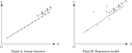
Figure 1.1 A function (panel A) compared to a regression model (panel B)

A consumption model explains the level of consumption in response to changes in income. This model is a simplification of reality. For example, it does not take into account the role of wealth on consumption. A more elaborate model would include other pertinent factors to improve the estimation and prediction of consumption.

Although this model is a good starting point, it is not a precise replication of reality. Nevertheless, it is similar to consumption functions in many introductory macroeconomics textbooks. As such, it serves a similar purpose: introduces the concept, clarifies application of the concept, and prepares for a more appropriate model.

Definition 1.2

A model is a simple representation of a phenomenon.

The extent to which a phenomenon is represented by a model is determined by the purpose of the model. Having more details does not necessarily make a model more desirable, in part because the purpose of a study affects the level of sophistication of the model.

Models need restrictions on their parameters to make sense. For example, the MPC has to be positive and less than one. A negative MPC means that as income increases, consumption decreases and eventually drops below subsistence level, while an MPC greater than one means that consumption at some point becomes larger than income. MPC values below zero or above one contradict reality and defy common sense. Therefore, economic theory restricts MPC to be between 0 and 1. In addition, negative values for the independent variable of income and the dependent variable of consumption are meaningless. Similarly, a negative subsistence level would be impossible. However, there are situations where the estimate for the subsistence level might turn out to be negative, but for the purpose of this example they can be ignored.

Income, consumption, MPC, and subsistence level are very different from each other. Consumption and income, the dependent and independent variables, are observable data. This means we can gather data on actual income and the consumption levels of a sample of people. The data are typically published and customarily represented in columnar formats. Subsistence consumption and MPC are called parameters. Parameters are unknown and have to be estimated. Although every nation has an MPC at any given point in time, the actual value is unknown, as is the case with the subsistence level of consumption (SLC). The parameters are estimated by the model using regression analysis. Parameters are also known as coefficients or slopes, in the jargon of regression analysis. The interpretation of coefficients and appropriate analysis are covered in Chapter 6.

Definition 1.3

A parameter is a characteristic of a population that is of interest. Parameters are constant and usually unknown.

Examples of parameters include the population mean, population variance, and regression coefficients. One of the main purposes of statistics is to obtain information from a sample that can be used to make inferences about population parameters. The estimated value obtained from a sample is called a statistic.

Definition 1.4

A statistic is a numerical value calculated from a sample that is variable and known.

The word statistic has several meanings depending on the context; two of its meanings are presented in the previous paragraph. The first use of the word refers to the science and the discipline of statistics. The second use is more specific and is based on the preceding definition. In the subject of statistics, we use statistics to make inference about parameters.

The slope and intercept terminologies used in geometry are also commonly used to refer to coefficients in regression analysis. In the consumption model, the corresponding analogy to geometry is that the MPC is the slope and the subsistence level is the intercept of the consumption line. According to this model, a dollar increase in income increases consumption by the magnitude of the MPC, which, by definition, is the slope of regression line. When income is zero, the amount of consumption is equal to the subsistence level, and, therefore, indicates the intercept.

The representative terms consumption and income used in Equation 1.1 only apply to this particular problem, which renders them inapplicable when the problem is changed. Consider a model that explains quantity demanded as a function of price of a good. If the price increases by $1, how much will the quantities demanded decrease? An attempt to write this question in the form of a model results in a stalemate for a typical economist wishing to stick to vocabulary that has economic meaning. In Equation 1.3, the problematic value is designated by a “?.” The value that replaces “?” answers, “if the price increases by $1, (how much) will the quantity demanded decrease?” The “(how much)” in the parenthesis does not have a defined economic name, thus, for the time being ...

Table of contents

• Cover
• Title
• Copyright
• Preface
• Acknowledgment
• Introduction
• Chapter 1. The Concept of Regression
• Chapter 2. The Method of Least Squares
• Chapter 3. Simple Linear Regression Using Software Packages
• Chapter 4. Multiple Regression
• Chapter 5. Goodness of Fit
• Chapter 6. Regression Coefficients
• Chapter 7. Causality: Correlation Is Not Causality
• Chapter 8. Qualitative Variables in Regression
• Chapter 9. Pitfalls of Regression Analysis
• Appendix
• Glossary of Terms
• Notes
• References
• Index
• Adpage
• Backcover