Design, Analysis and Optimization of Supply Chains

A System Dynamics Approach

William R. Killingsworth

• Publisher: Business Expert Press
• Year: 2011
• Print ISBN: 9781606492512
• eBook ISBN: 9781606492529
• Topic: Business
• Subtopic: Operations
• Index: Business

If you're an executive dealing with extended supply chains, you live with stress and worry. Almost everything made today is manufactured by large networks of companies. Hundreds, if not thousands, of companies provide components, subassemblies, and major assemblies to a final manufacturer or integrator. These large distributed supply chains have created problems and headaches for many industries.

This book can help you prevent lost sales due to inventory shortages, high costs due to large inventories, work stoppage due to loss of a key supplier, and supply problems that may be causing a late introduction of a new product.

Today's supply chains are not only highly complex in terms of the number of companies involved but also dynamically complex in that their behavior and performance variations over time range from "hard to comprehend" to baffling. It's no wonder that management is so difficult and challenging. Developing an intuitive grasp of supply chain dynamic behavior is the first step in driving performance improvement.

In this book, a system dynamics framework for analyzing complex supply chain performance is presented. The feedback nature of supply chains is demonstrated and dynamic simulation models are used to examine the counterintuitive behavior that arises from time delays, lack of information, and incorrect planning assumptions. The benefits of establishing push–pull boundaries in supply chains are shown to provide increased customer service levels with reduced costs. Dynamic supply chain models are used to determine product lifecycle costs and the impacts of improved reliability on lifecycle costs. A basic system dynamics model is used to show that the goal of a "lean and mean" supply chain can be dangerous in periods of economic, political, and climatic volatility, and strategies are developed for improved supply chain management and performance.

Chapter 1

A Static Versus a Dynamic View of Supply Chains

Introduction

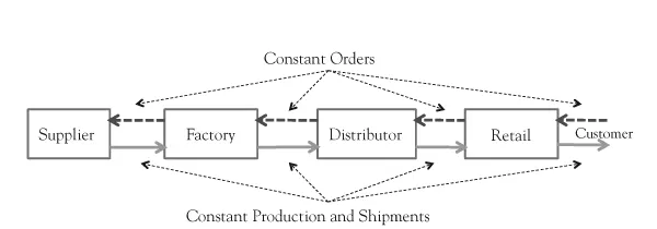
Supply chains are often viewed as a simple, static system with constant demand, constant orders, and constant production. Generally, these supply chains are viewed as a simple linear “chain” of participants such as a retail store, a distributor, a factory, and perhaps a key supplier to the factory as shown in Figure 1.1.

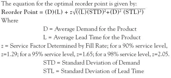
At the next level of complexity, these linear chains are viewed as a static stochastic system having constant means and constant standard deviations for demand, orders, and production. This statistically based view of the static supply chain resulted in several well-known optimization solutions such as the economic order quantity and optimum reorder points.¹ These optimal solutions determine an ordering strategy that minimizes cost for an assumed level of customer service. The well-known equation for the reorder point, as shown here, includes the demand expected over the lead time as the key component and a safety factor that reflects uncertainty in demand and lead time.

Figure 1.1. A basic review of a static supply chain.

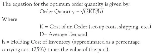
Thus, once the reorder point is reached, the order quantity is proportional to demand and the cost of an order and is inversely proportional to the holding cost. Thus, if ordering costs are high, then the equation tends to order a higher quantity and reduce the number of orders. On the other hand, if an item is expensive with high holding costs, then the equation tends to order a lower quantity and reduce inventory holding costs. These equations provide useful guidance and insight but, in a dynamic system with time delays and lack of information sharing, they are as likely to create the bullwhip as other ordering processes.

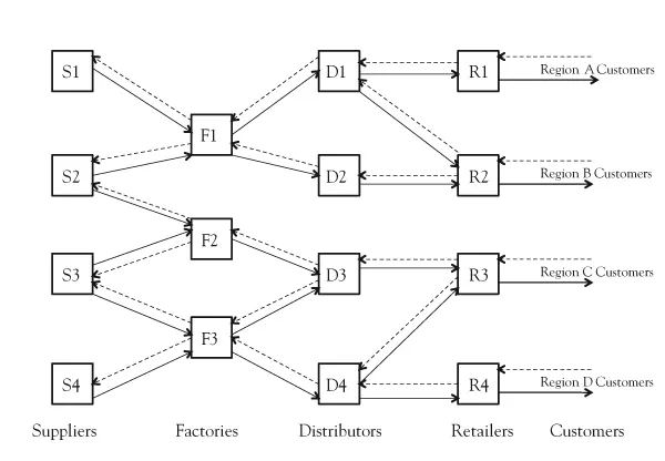
In today’s supply chains, complexity arises not only from dynamics but also from the sheer number of participating entities. The typical supply chain involves hundreds, if not thousands, of suppliers, multiple factories, numerous distribution centers, and customers spread across the globe. These supply chains are often depicted as shown in Figure 1.2. Although more complex, they are again primarily analyzed in a static mode of constant flows of orders and material or with constant statistics. These more complex networks can also be analyzed for minimum cost at a specified level of customer service. These optimization solutions, however, fail to predict supply chain dynamics and the substantial swings that can occur in inventories, orders, and shipments as in the bullwhip. In order to understand and correct those problems, a dynamic view and model of the supply chain is required.

Figure 1.2. A more complex view of a static supply chain. Multiple suppliers supplying multiple factories with multiple distribution centers and multiple regions of customers.

System Dynamics

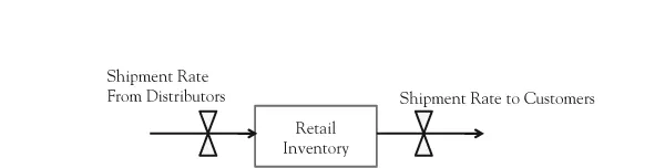
System dynamics is a modeling and simulation approach to studying the behavior of complex systems over time. The approach was developed by Jay Forrester at MIT in the mid-1950s and the 1960s. System dynamics focuses on internal feedback loops and the time delays that affect the dynamics of the entire system. Forrester treated a complex system as a system of stocks and flows where the flows, or rates of change, were determined via feedback loops. Forrester’s key insight was that changes in stocks (sometimes called levels) occur only through associated rates of change, not through a correlation with other variables. A system dynamics model focuses on those key rates that increase or reduce a stock or level over time. For example, a retailer’s inventory is reduced by the shipment rate to customers and is increased by shipments received from a distributor. The dynamics of the inventory level are thus the accumulation (or, mathematically, the integration) of all flows into and out of the retailer’s inventory. This structure is often shown as pictured in Figure 1.3.

In the simulation of a system dynamics model, given an initial condition for the retail inventory, future inventory levels are developed by mathematically integrating these two flows over a sequence of discrete time steps. Thus the inventory after a small time interval is equal to the initial inventory plus the time step, Δt, multiplied by the shipment rate from distributors during that time interval, minus the time step multiplied by the shipment rate to customers during that time interval:

I1 = I0 + (Δt)(Shipment Rate from Distributors)01 – (Δt)(Shipment Rate to Customers)01

Figure 1.3. Illustration of rates and levels.

The next calculation for the inventory level is then given as:

I2 = I1 + (Δt)(Shipment Rate from Distributors)12 – (Δt)(Shipment Rate to Customers)12

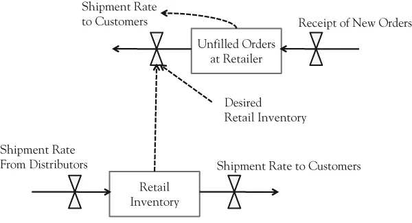
For the simulation, Δt must be considerably shorter than the time delays within the system, such as shipping times, order processing times, and so forth. Since retailers may not always have adequate inventory for immediate shipment, Forrester’s model necessarily included a level for unfilled orders. This level depended on an inflow rate of new orders and a reducing rate of shipments to customers. The form of the equation is similar to the previous one.

U1 = U0 + (Δt)(Receipt of New Orders)01 – (Δt)(Shipment Rate to Customers)01

and

U2 = U1 + (Δt)(Receipt of New Orders)12 – (Δt)(Shipment Rate to Customers)12

In the simulation, other equations are used to calculate the various rates. These rates typically depend on stocks or levels in the model. For example, in Forrester’s model, the shipment rate to customers is dependent on the level of unfilled orders and the physical availability of inventory at the distributor, in this case expressed as the square root of the ratio of inventory to desired inventory. This is shown in Figure 1.4. In many cases, the desired inventory is a multiple of average demand, for example, 2 weeks of average sales or a month of sales. This averaging of sales is only one way in which time delays are included in the model. Other delays relate to purchasing processes, shipping times, and factory-production lead times.

System dynamics, by focusing on rates of change, feedback of information, and time delays, creates models that are difference equations for nonlinear differential equations. The stocks or levels are the state variables of the system. This approach enables the models to capture and replicate counterintuitive, and at times baffling, nonlinear behavior of systems, such as the bullwhip effect.

Figure 1.4. Determination of rates.

Figure 1.5. Simple feedback model.

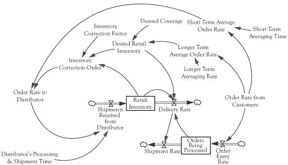
A simple model as shown in Figure 1.5 can also help illustrate model development and simulation. Whereas Forrester’s model included three stages in a supply chain—factory, distributor, and retailer—this illustrative model includes only the retail sector. In the model, a retailer receives orders from customers. Shipments occur after a day or so of processing but only if inventory is available. In terms of assessing the inventory position, the retailer compares the current inventory with a desired level of inventory. As inventory falls below the desired level, the retailer slows shipments to avoid running out of inventory. The retailer tries to maintain 2 weeks of average sales as the desired level of inventory, often termed a 2-week coverage. To be conservative in this determination, the retailer averages sales over a 4-week period, smoothing out any potentially misleading short-term fluctuations. The desired inventory is then twice this 4-week average. The retailer’s order to the distributor is composed of the recent order rate plus a term that is proportional to the difference between the inventory and the desired inventory. This second component reflects a corrective feedback mechanism that drives inventory toward the desired level. This type of corrective action is a key feature of supply chain management and is widely reflected in the real world. The ability to capture this corrective feedback is a key aspect of system dynamics. It is assumed in this simple model that inventory is always available at the distributor so that after an average 4-week processing and shipment delay, the ordered shipments arrive at the retailer.

If the order rate from customers is constant at 10 per week, the model with the corrective feedback maintai...

Table of contents

• Title Page
• Copyright Page
• Contents
• Acknowledgments
• Introduction
• Chapter 1. A Static Versus a Dynamic View of Supply Chains
• Chapter 2. The Dynamics of the Supply Process for High-Value Spare Parts
• Chapter 3. The Dynamics of Multitier, Multichannel Supply Chains
• Chapter 4. Using System Dynamics to Evaluate a Push-Pull Inventory Optimization Strategy for Multitier, Multichannel Supply Chains
• Chapter 5. Using System Dynamics to Estimate Reductions in Life-Cycle Costs Arising From Investments in Improved Reliability
• Chapter 6. The Role of Overhaul in Reducing Life-Cycle Costs and Maximizing the Return on Investments to Improve Reliability
• Chapter 7. Future Supply Chains and System Dynamics
• Notes
• References