Transportation Network Modeling and Calibration

Mansoureh Jeihani, Anam Ardeshiri

• Publisher: Momentum Press
• Year: 2017
• ISBN:
  9781606508947
• Topic: Tecnologia e ingegneria
• Subtopic: Trasporto e navigazione

Transportation scientists employ modeling and simulation techniques to capture the complexities of transportation systems and develop and assess solutions to alleviate existing and future transportation-related problems. This book introduces transportation engineering students and junior engineers to the concept of transportation network modeling, network coding, model calibration and validation, and model evaluation. Travel demand models are sensitive to demographic changes and can explain and forecast how a new transportation supply system leads to a new transportation demand pattern. This book also describes how demand models evolved from trip-based to the newer generation of activity-based and agent-based to overcome some of the shortcomings of the four-step approach and improve models' prediction power.

CHAPTER 1

INTRODUCTION

Transportation is the means to reach a destination. It facilitates people and goods being where they need to be at a certain time. Transportation science is established to illustrate and evaluate the quality of people and goods’ movement along transportation infrastructure of all shapes, including ground, rail, waterway, air, and pipeline. Similarly, many other facts evolve in the rapidly changing world, and travel patterns and travelers’ behavior are constantly transforming to adapt to today’s lifestyle and respond to new transportation needs. Transportation models are capable of calculating traffic consequences, including travel delays, queue backups, environmental impacts, energy consumption, and crash rate.

The first step of modeling transportation is to develop a transportation network of the study area as a setting for people to travel. A transportation network comprises several items, with each representing one real-world element in our daily travel life. Network links denote urban streets, while nodes represent street junctions. Vehicles and travelers are moving objects in a transportation network in the direction(s) defined for the links. A transportation network shows the origin and destination of traffic, from which node vehicles can enter and exit the network. All feasible and allowed movements or parking restrictions (by time of day) are reflected in the transportation model. The notion of a supernetwork indicates the basic transportation network augmented with dummy links. This concept is beneficial when combining travel demand problems in different stages and solving a joint equilibrium problem. In summary, what is necessary in network modeling may comprise the following:

• Direction of flow

• Capacity of roadway per direction (maximum flow rate)

• Traffic control system at junctions or intersections

• Traffic volumes

• Pedestrian and bike activities

• Heavy vehicles

• Traveler awareness system (about travel information)

• Traffic mix, such as car, bus, and bicycle

• Link speed or travel time

• Link interaction (travel time versus volume of the link)

This chapter begins with a review of transportation demand, supply, and equilibrium concepts. Later, it explains the key components of transportation networks and their roles in the models.

1.1 TRANSPORTATION DEMAND

The public definition of transportation demand is the need for transportation services that generate movements of people and freight. Demand for transportation is the willingness to pay for transportation services and how this willingness changes when the price changes. The economic definition of transportation demand is the relationship between the quantity of transportation services demanded (consumed) and the price people are willing to pay for it. This relationship is shown with a curve. The demand curve is the downward slope as presented in Figure 1.1, which presents the quantity demanded versus price. When the price of transportation service increases, demand decreases. Examples of quantity demanded are vehicle per hour, number of passengers per day, and tons per day (for freight).

1.2 TRANSPORTATION SUPPLY

The capacity of infrastructure and transportation mode over a geographically defined transportation system and a specific period of time is called transportation supply. The economic definition of transportation supply is the relationship between the quantity of transportation services supplied (offered) and the price charged for it. The supply curve is an upward slope as presented in Figure 1.1, which presents the quantity demanded versus price. Examples of the quantity supplied are vehicle per hour, number of passengers per day, and tons per day (for freight).

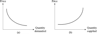
Figure 1.1. (a) Demand curve (b) Supply curve.

1.3 EQUILIBRIUM

Equilibrium is defined as the price in which the quantity demanded and the quantity supplied is equal. Figure 1.2 presents the equilibrium (P*, Q*). In other words, equilibrium is the point where the price of transportation is just right, so that the quantity demanded is entirely supplied. If the price is higher than P*, then the quantity supplied is more than the quantity demanded, resulting in a surplus. If the price is lower than P*, the quantity demanded is more than the quantity supplied, resulting in a deficit.

When demand increases (decreases), the demand curve shifts up (down), and so, the equilibrium price and quantity both increase (decrease), as presented in Figure 1.3. It means that more (less) transportation services are purchased at a higher (lower) price. As presented in Figure 1.3, when supply increases (decreases), the supply curve shifts to the right (left), reducing (increasing) the equilibrium price while the equilibrium quantity increases (decreases). When both the demand and supply increase, the equilibrium quantity increases, but the price might increase, decrease, or stay the same, depending on the amount of increase in demand and supply.

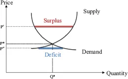
Figure 1.2. Equilibrium, surplus, and deficit.

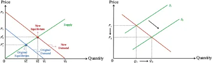
Figure 1.3. Change in equilibrium when (a) demand increases (b) supply increases.

1.4 TRANSPORTATION DEMAND AND SUPPLY MODELS

Transportation modeling comprises of modeling models, both supply and demand sides of transportation. While the supply side is less dynamic and more predictable, modeling the transportation demand can be very challenging considering the interaction between drivers and reaction to the change in other factors, such as weather, work zone, school zone, and incident. Transportation demand models formulate and predict transportation demand. The demand is usually described by origin, destination, and mode, time, and path of travel. The demand may be estimated by the trip region (e.g., home-based) or by special purposes (e.g., work trips) or destinations (e.g., airport).

Transportation supply models predict the per...