1.1 Why study numerical methods?
A fundamental questions one should ask before spending time and effort learning a new subject is “Why should I bother?”. Aside from the fun of learning something new, the need for this course arises from the fact that most mathematics done in practice (therefore by engineers and scientists) is now done on a computer. For example, it is common in engineering to need to solve more than 1 million linear equations simultaneously, and even though we know how to do this ‘by hand’ with Gaussian elimination, computers can be used to reduce calculation time from years (if you tried to do it by hand - but you would probably make a mistake!) to minutes or even seconds. Furthermore, since a computer has a finite number system and each operation requires a physical change in the computer system, the idea of having infinite processes such as limits (and therefore derivatives and integrals) or summing infinite series (which occur in calculating sin, cos, and exponential functions for example) cannot be performed on a computer. However, we still need to be able to calculate these important quantities, and thus we need to be able to approximate these processes and functions. Often in scientific computing, there are obvious ways to do approximations; however it is usually the case that the obvious ways are not the best ways. This raises some fundamental questions:
- – How do we best approximate these important mathematical processes/operations?
- – How accurate are our approximations?
- – How efficient are our approximations?
It should be no surprise that we want to quantify accuracy as much as possible. Moreover, when the method fails, we want to know why it fails. In this course, we will see how to rigorously analyze the accuracy of several numerical methods. Concerning efficiency, we can never have the answer fast enough, but often there is a trade-off between speed and accuracy. Hence we also analyze efficiency, so that we can ‘choose wisely’ when selecting an algorithm.
Thus, to put it succinctly, the purpose of this course is to
- – Introduce students to some basic numerical methods for using mathematical methods on the computer.
- – Analyze these methods for accuracy and efficiency.
- – Implement these methods and use them to solve problems.
1.2 Terminology
Here are some important definitions:
- – A numerical method is any mathematical technique used to approximate a solution to a mathematical problem.
Common examples of numerical methods you may already know include Newton’s method for root-finding and Gaussian elimination for solving systems of linear equations.
- – An analytical solution is a closed form expression for unknown variables in terms of the known variables.
For example, suppose we want to solve the problem
for a given (known) a, b, and c. The quadratic formula tells us the solutions are
Each of these solutions is an analytical solution to the problem.
- – A numerical solution is a number that approximates a solution to a mathematical problem in one particular instance.
For the example above for finding the roots of a quadratic polynomial, to use a numerical method such as Newton’s method, we would need to start with a specified a,b, and c. Suppose we choose a = 1, b = -2, c = -1, and ran Newton’s method with an initial guess of x0 = 0. This returns the numerical solution of x = -0.414213562373095.
There are two clear disadvantages to numerical solutions compared to analytic solutions. First, they only work for a particular instance of a problem, and second, they are not as accurate. It turns out this solution is accurate to 16 digits (which is approximately the standard number of digits a computer stores for any number), but if you needed accuracy to 20 digits then you need to go through some serious work to get it. But many other numerical methods will only give ‘a few’ digits of accuracy in a reasonable amount of time.
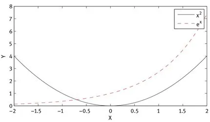
On the other hand, there is a clear advantage to using numerical methods in that they can solve many problems that we cannot solve analytically. For example, can you analytically find the solution to
Probably you cannot. But if we look at the plots of y = ex and y = x2 in Figure 1.1, it is clear that a solution exists. If we run Newton’s method to find the zero of x2 – ex, it takes no time at all to arrive at the approximation (correct to 16 digits) x = -0.703467422498392. In this sense, numerical methods can be an enabling technology.
Fig. 1.1. Plots of ex and x2.
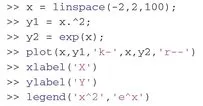
The plot in Figure 1.1 was created with the following commands:
Some notes on these commands:
- – The function linspace (a, b, n) creates a vector of n equally spaced points from a to b.
- – In the definition of y1, we use a period in front of the power symbol. This denotes a ‘vector operation’. ...