eBook - ePub
Using and Understanding Medical Statistics
- 338 pages
- English
- ePUB (mobile friendly)
- Available on iOS & Android
eBook - ePub
Using and Understanding Medical Statistics
About this book
The fifth revised edition of this highly successful book presents the most extensive enhancement since Using and Understanding Medical Statistics was first published 30 years ago. Without question, the single greatest change has been the inclusion of source code, together with selected output, for the award-winning, open-source, statistical package known as R. This innovation has enabled the authors to de-emphasize formulae and calculations, and let software do all of the 'heavy lifting'. This edition also introduces readers to several graphical statistical tools, such as Q-Q plots to check normality, residual plots for multiple regression models, funnel plots to detect publication bias in a meta-analysis and Bland-Altman plots for assessing agreement in clinical measurements. New examples that better serve the expository goals have been added to a half-dozen chapters. In addition, there are new sections describing exact confidence bands for the Kaplan-Meier estimator, as well as negative binomial and zero-inflated Poisson regression models for over-dispersed count data. The end result is not only an excellent introduction to medical statistics, but also an invaluable reference for every discerning reader of medical research literature.
Trusted by 375,005 students
Access to over 1.5 million titles for a fair monthly price.
Study more efficiently using our study tools.
Information
1
______________________
Basic Concepts
1.1 Introduction
A brief glance through almost any recently published medical journal will show that statistical methods play an increasingly visible role in modern medical research. At the very least, most research papers quote (at least) one ‘p value’ to underscore the ‘significance’ of the results that the authors wish to communicate. At the same time, many papers are now presenting the results of relatively sophisticated ‘multi-factor’ statistical analyses of complex sets of medical data. This proliferation in the use of statistical methods has also been paralleled by a commensurate involvement of professionally trained statisticians in medical research as consultants to and collaborators with the medical researchers themselves.
The primary purpose of this book is to provide medical researchers with sufficient understanding to enable them to read, intelligently, statistical methods and discussion appearing in medical journals. At the same time, we have tried to provide the means for researchers to undertake many of the analyses we describe on their own, if this is their wish. And by presenting statistics from this perspective, we hope to extend and improve the common base of understanding that is necessary whenever medical researchers and statisticians interact.
It seems obvious to us that statisticians involved in medical research need to have some understanding of the related medical knowledge. We also believe that in order to benefit from statistical advice, medical researchers require some understanding of the subject of statistics. This first chapter provides a brief introduction to some of the terms and symbols that recur throughout the book. It also establishes what statisticians talk about (random variables, probability distributions) and how they talk about these concepts (standard notation). We are very aware that this material is difficult to motivate; it seems so distant from the core and purpose of medical statistics. Nevertheless, ‘these dry bones’ provide a skeleton that allows the rest of the book to be more precise about statistics and medical research than would otherwise be possible. Therefore, we urge the reader to forbear with these beginnings, and read beyond the end of chapter 1 to see whether we do not put flesh onto these dry bones.
1.2 Random Variables, Probability Distributions and Some Standard Notation
Most statistical work is based on the concept of a random variable. This is a quantity that, theoretically, may assume a wide variety of actual values, although in any particular realization we only observe a single value. Measurements are common examples of random variables; take the weights of individuals belonging to a well-defined group of patients, for example. Regardless of the characteristic that determines membership in the group, the actual weight of each individual patient is almost certain to differ from that of other group members. Thus, a statistician might refer to the random variable representing the weight of individual patients in the group or population of interest. Another example of a random variable might be a person’s systolic blood pressure; the variation in this measurement from individual to individual is frequently quite substantial.
To represent a particular random variable, statisticians generally use an upper case Roman letter, say X or Y. The particular value that this random variable represents in a specific instance is often denoted by the corresponding lower case Roman letter, say x or y. The probability distribution (usually shortened to the distribution) of any random variable can be thought of as a specification of all possible numerical values of the random variable, together with an indication of the frequency with which each numerical value occurs in the population of interest.
It is common statistical shorthand to use subscripted letters - x1, x2, …, xn, for example - to specify a set of observed values of the random variable X. The corresponding notation for the associated set of random variables is Xi, i = 1, 2, …, n, where Xi indicates that the random variable of interest is labelled X and the symbols i = 1,2,…, n specify the possible values of the subscripts on X. Similarly, using n as the final subscript in the set simply indicates that the size of the set may vary from one instance to another, but in each particular instance it will be a fixed number.
Subscripted letters constitute extremely useful notation for the statistician, who must specify precise formulae that will subsequently be applied in particular situations that vary enormously. At this point it is also convenient to introduce the use of ∑, the upper case Greek letter sigma. In mathematics, ∑ represents summation. To specify the sum X1 + X2 + X3, we would simply write

This expression specifies that the subscript i should take the values 1, 2 and 3 in turn, and we should sum the resulting variables. For a fixed but unspecified number of variables, say n, the sum X1 + X2 + … + Xn would be denoted by

A set of values x1, x2, …, xn is called a sample from the population of all possible occurrences of X. In general, statistical procedures that use such a sample assume that it is a random sample from the population. The random sample assumption is imposed to ensure that the characteristics of the sample reflect those of the entire population, of which the sample is often only a small fraction.
There are two types of random variables. If we overlook certain technicalities, a discrete random variable is commonly defined as one for which we can write down all its possible values and their corresponding frequencies of occurrence. In contrast, continuous random variables are measured on an interval scale, and the variable can assume any value on the scale. Of course, the instruments that we use to measure experimental quantities, e.g., blood pressure, acid concentration, weight, height, etc., have a finite resolution, but it is convenient to suppose, in such situations, that this limitation does not prevent us from observing any plausible measurement. Furthermore, the notation that statisticians have adopted to represent all possible values belonging to a given interval is to enclose the end-points of the interval in parentheses. Thus, (a, b) specifies the set of all possible values between a and b, and the symbolic statement a < X < b means that the random variable X takes a value within the interval specified by (a, b).
The probability distribution of a random variable is often illustrated by means of a histogram or bar graph. This is a picture that indicates how frequently each value of the random variable occurs, either in a sample or in the corresponding population. If the random variable is discrete, the picture is generally a simple one to draw and to understand. Figure 1.1a shows a histogram for random variable S, which represents the sum of the showing faces of two fair dice. Notice that there are exactly 11 possible values for S. In contrast to this situation, the histogram for a continuous random variable X, say systolic blood pressure, is somewhat more difficult to draw and to understand. One such histogram is presented in figure 1.1b. Since the picture is intended to show both the possible values of X and also the frequency with which they arise, each rectangular block in the graph has an area equal to the proportion of the sample represented by all outcomes belonging to the interval on the base of the block. This has the effect of equating frequency, or probability of occurrence, with area and is known as the area = probability equation for continuous random variables.
To a statistician, histograms are simply an approximate picture of the mathematical way of describing the distribution of a continuous random variable. A more accurate representation of the distribution is obtained by using the equation of a curve that can best be thought of as a ‘smooth histogram’; such a curve is called a probability density function. A more convenient term, and one that we intend to use, is probability curve.
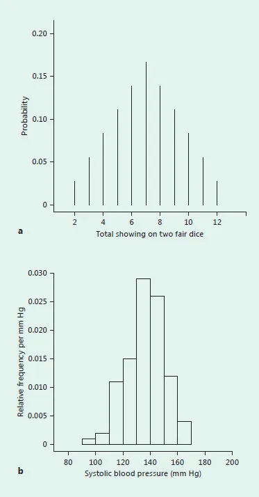
Fig. 1.1. Histograms of random variables. a The discrete random variable S, representing the sum of the showing faces on two fair dice. b One hundred observations on the continuous random variable X, representing systolic blood pressure.
Figure 1.2a shows the probability curve, or smooth histogram, for continuous random variable X that we used above to represent systolic blood pressure. This curve is, in fact, the probability curve that has the characteristic shape and equation known as a normal distribution. Random variables that have a normal distribution will recur in subsequent chapters, and we intend to explain their properties and uses in more detail at that time. For the present, however, we want to concentrate on the concept of the area = probability equation. Figure 1.2b shows two shaded areas. One is the area below the curve and above the interval (110, 130). Recall that the symbol (110, 130) represents all blood pressure measurements between 110 and 130 mm Hg. This area can be calculated mathematically, and in this particular example the value is 0.322. To represent this calculation in a symbolic statement we would write Pr(110 < X < 130) = 0.322; the equation states that the probability that X, a systolic blood pressure measurement in the population, is between 110 and 130 mm Hg is equal to 0.322.
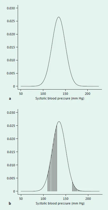
Fig. 1.2. A probability curve for the continuous random variable X, representing systolic blood pressure as a smooth histogram (a) with shaded areas corresponding to Pr(110 < X < 130) and Pr(X > 165)(b).
The second shaded area in figure 1.2b is the area below the probability curve corresponding to values of X in the interval (165, ∞), i.e., the probability that a systolic blood pressure measurement in the population exceeds 165 mm Hg. By means of certain calculations we can determine that, for this specific example, the probability that systolic blood pressure exceeds 165 mm Hg is 0.023; the concise mathematical description of this calculation is simply Pr(X > 165) = 0.023.
The second shaded area in figure 1.2b is the area below the probability curve corresponding to values of X in the interval (165, ∞), i.e., the probability that a systolic blood pressure measurement in the population exceeds 165 mm Hg. By means of certain calculations we can determine that, for this specific example, the probability that systolic blood pressure exceeds 165 mm Hg is 0.023; the concise mathematical description of this calculation is simply Pr(X > 165) = 0.023.
Although the probability curve makes it easy to picture the equality of area and probability, it is of little direct use for actually calculating probabilities, since areas cannot be read directly from a picture or sketch. Instead, we need a related function called the cumulative probability curve. Figure 1.3 presents the cumulative probability curve for the normal distribution shown in figure 1.2a. The horizontal axis represents the possible values of the random variable X; the vertical axis is a probability scale with values ranging from 0 to 1. The cumulative probability curve specifies, for each value a on the horizontal axis, the probability that the random variable X takes a value which is at most a, i.e., Pr(X ≤ a). This probability is precisely the area below the probability curve corresponding to values of X in the interval (-∞, a). In particular, if a = ∞, i.e., Pr(-∞ < X < ∞), the value of the cumulative probability curve is 1, indicating that X is certain to assume some value in the interval (-∞ < X < ∞). In fact, this result is a necessary property of all cumulative probability curves, an...
Table of contents
- Cover Page
- Front Matter
- 1 Basic Concepts
- 2 Tests of Significance
- 3 Fisher’s Test for 2 × 2 Contingency Tables
- 4 Approximate Significance Tests for Contingency Tables
- 5 Some Warnings concerning 2 × 2 Tables
- 6 Kaplan-Meier or ‘Actuarial’ Survival Curves
- 7 The Log-Rank or Mantel-Haenszel Test for Comparing Survival Curves
- 8 An Introduction to the Normal Distribution
- 9 Analyzing Normally Distributed Data
- 10 Linear Regression Models for Medical Data
- 11 Binary Logistic Regression
- 12 Regression Models for Count Data
- 13 Proportional Hazards Regression
- 14 The Analysis of Longitudinal Data
- 15 Analysis of Variance
- 16 Data Analysis
- 17 The Question of Sample Size
- 18 The Design of Clinical Trials
- 19 Further Comments regarding Clinical Trials
- 20 Meta-Analysis
- 21 Epidemiological Applications
- 22 Diagnostic Tests
- 23 Agreement and Reliability
- References
- Subject Index
Frequently asked questions
Yes, you can cancel anytime from the Subscription tab in your account settings on the Perlego website. Your subscription will stay active until the end of your current billing period. Learn how to cancel your subscription
No, books cannot be downloaded as external files, such as PDFs, for use outside of Perlego. However, you can download books within the Perlego app for offline reading on mobile or tablet. Learn how to download books offline
Perlego offers two plans: Essential and Complete
- Essential is ideal for learners and professionals who enjoy exploring a wide range of subjects. Access the Essential Library with 800,000+ trusted titles and best-sellers across business, personal growth, and the humanities. Includes unlimited reading time and Standard Read Aloud voice.
- Complete: Perfect for advanced learners and researchers needing full, unrestricted access. Unlock 1.5M+ books across hundreds of subjects, including academic and specialized titles. The Complete Plan also includes advanced features like Premium Read Aloud and Research Assistant.
We are an online textbook subscription service, where you can get access to an entire online library for less than the price of a single book per month. With over 1.5 million books across 990+ topics, we’ve got you covered! Learn about our mission
Look out for the read-aloud symbol on your next book to see if you can listen to it. The read-aloud tool reads text aloud for you, highlighting the text as it is being read. You can pause it, speed it up and slow it down. Learn more about Read Aloud
Yes! You can use the Perlego app on both iOS and Android devices to read anytime, anywhere — even offline. Perfect for commutes or when you’re on the go.
Please note we cannot support devices running on iOS 13 and Android 7 or earlier. Learn more about using the app
Please note we cannot support devices running on iOS 13 and Android 7 or earlier. Learn more about using the app
Yes, you can access Using and Understanding Medical Statistics by D. E. Matthews,V. T. Farewell,D.E., Matthews,V.T., Farewell in PDF and/or ePUB format, as well as other popular books in Medicine & Communication Studies. We have over 1.5 million books available in our catalogue for you to explore.