Dynamic Models in Biology

Stephen P. Ellner, John Guckenheimer

• Publisher: Princeton University Press
• Year: 2011
• ISBN:
  9781400840960
• Topic: Biological Sciences
• Subtopic: Biology
• Index: Biological Sciences

From controlling disease outbreaks to predicting heart attacks, dynamic models are increasingly crucial for understanding biological processes. Many universities are starting undergraduate programs in computational biology to introduce students to this rapidly growing field. In Dynamic Models in Biology, the first text on dynamic models specifically written for undergraduate students in the biological sciences, ecologist Stephen Ellner and mathematician John Guckenheimer teach students how to understand, build, and use dynamic models in biology.
Developed from a course taught by Ellner and Guckenheimer at Cornell University, the book is organized around biological applications, with mathematics and computing developed through case studies at the molecular, cellular, and population levels. The authors cover both simple analytic models--the sort usually found in mathematical biology texts--and the complex computational models now used by both biologists and mathematicians.
Linked to a Web site with computer-lab materials and exercises, Dynamic Models in Biology is a major new introduction to dynamic models for students in the biological sciences, mathematics, and engineering.

1	What Are Dynamic Models?

Dynamic models are simplified representations of some real-world entity, in equations or computer code. They are intended to mimic some essential features of the study system while leaving out inessentials. The models are called dynamic because they describe how system properties change over time: a gene’s expression level, the abundance of an endangered species, the mercury level in different organs within an individual, and so on. Mathematics, computation, and computer simulation are used to analyze models, producing results that say something about the study system. We study the process of formulating models, analyzing them, and drawing conclusions. The construction of successful models is constrained by what we can measure, either to estimate parameters that are part of the model formulation or to validate model predictions. Dynamic models are invaluable because they allow us to examine relationships that could not be sorted out by purely experimental methods, and to make forecasts that cannot be made strictly by extrapolating from data.

Dynamic models in biology are diverse in several different ways, including

• the area of biology being investigated (cellular physiology, disease prevalence, extinction of endangered species, and so on),

• the mathematical setting of the model (continuous or discrete time and model variables, finite- or infinite-dimensional model variables, deterministic or stochastic models, and so on),

• methods for studying the model (mathematical analysis, computer simulation, parameter estimation and validation from data, and so on),

• the purpose of the model (“fundamental” science, medicine, environmental management, and so on).

Throughout this book we use a wide-ranging set of case studies to illustrate different aspects of models and modeling. In this introductory chapter we describe and give examples of different types of models and their uses. We begin by describing the principles that we use to formulate dynamic models, and then give examples that illustrate the range of model types and applications. We do only a little bit of mathematics, some algebra showing how a model for enzyme kinetics can be replaced by a much simpler model which can be solved explicitly. We close with a general discussion of the final “dimension” listed above—the different purposes that dynamic models serve in biology. This chapter is intended to provide a basic conceptual framework for the study of dynamic models—what are they? how do they differ from other kinds of models? where do they come from?—and to flesh out the framework with some specific examples. Subsequent chapters are organized around important types of dynamic models that provide essential analytical tools, and examples of significant applications that use these methods. We explain just enough of the mathematics to understand and interpret how it is used to study the models, relying upon computers to do the heavy lifting of mathematical computations.

1.1 Descriptive versus Mechanistic Models

Salmon stocks in the Pacific Northwest have been in steady decline for several decades. In order to reverse this trend, we need to know what’s causing it. Figure 1.1 shows data on salmon populations on the Thomson River in British Columbia (Bradford and Irvine 2000). Figure 1.2 presents the results from statistical analyses in which data from individual streams are used to examine how the rate of decline is affected by variables describing the impacts of humans on the surrounding habitat. Straight lines fitted to the data—called a linear regression model—provide a concise summary of the overall trends and quantify how strongly the rate of decline is affected by land use and road density. These are examples of descriptive models—a quantitative summary of the observed relationships among a set of measured variables.

Figure 1.2 provides very useful information, and descriptive models such as these are indispensable in biology, but it also has its limitations.

• It says nothing about why the variables are related the way they are. Based on the results we might decide that reducing road density would help the salmon, but maybe road density is just an indicator for something else that is the actual problem, such as fertilizer runoff from agriculture.

• We can only be confident that it applies to the river where the data come from. It might apply to other rivers in the same region, and even to other regions—but it might not. This is sometimes expressed as the “eleventh commandment for statisticians”: Thou Shalt not Extrapolate Beyond the Range of Thy Data. The commandment is necessary because we often want to extrapolate beyond the range of our data in order to make useful predictions—for example, how salmon stocks might respond if road density were reduced.

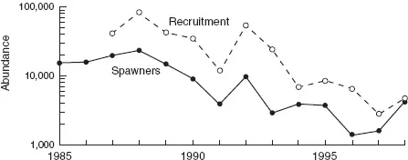
Figure 1.1 Decline in Coho salmon stocks on the Thomson River, BC (from Bradford and Irvine 2000).

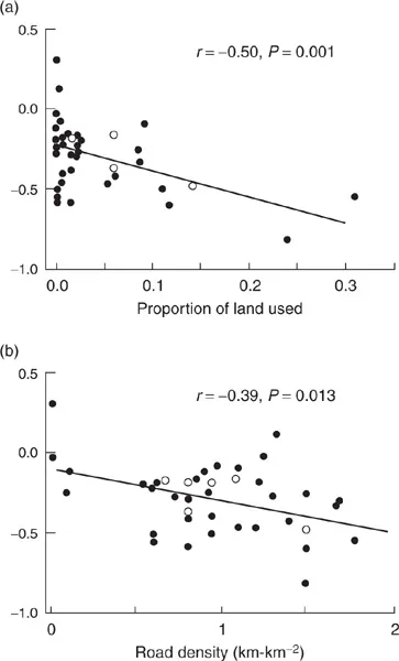
Figure 1.2 Rate of decline on individual streams related to habitat variables (from Bradford and Irvine 2000).

The second limitation is related to the first. If we knew why the observed relationships hold in this particular location, we would have a basis for inferring where and when else they can be expected to hold.

In contrast, a dynamic model is mechanistic, meaning that it is built by explicitly considering the processes that produce our observations. Relationships between variables emerge from the model as the result of the underlying process. A dynamic model has two essential components:

• A short list of state variables that are taken to be sufficient for summarizing the properties of interest in the study system, and predicting how those properties will change over time. These are combined into a state vector X (a vector is an ordered list of numbers).

• The dynamic equations: a set of equations or rules specifying how the state variables change over time, as a function of the current and past values of the state variables.

A model’s dynamic equations may also include a vector E of exogenous variables that describe the system’s environment—attributes of the external world that change over time and affect the study system, but are not affected by it.

Because it is built up from the underlying causal processes, a dynamic model expands the Range of Thy Data to include any circumstances where the same processes can be presumed to operate. This is particularly important for projecting how a system will behave in the future. If there are long-term trends, the system may soon exceed the limits of current data. With a dynamic model, we still have a basis for predicting the long-term consequences of the processes currently operating in the study system.

1.2 Chinook Salmon

As a first example, here is a highly simplified dynamic model for the abundance of Chinook salmon stocks, based on some models involved in planning for conservation and management of stocks in the Columbia River basin (Oosterhout and Mundy 2001, Wilson 2003). Most fish return as adults to spawn in the stream where they were born; we will pretend for now that all of them do, so that we can model on a stream-by-stream basis. The state variable in the model for an individual stream is S(t), the number of females spawning there in year t. The biology behind the simple models is as follows.

1. Fish return to spawn at age four or five, and then die. Of those that do return, roughly 28% return at age four, 72% at age five; this actually varies somewhat over time, but it turns out not to matter much for long-term population trends.

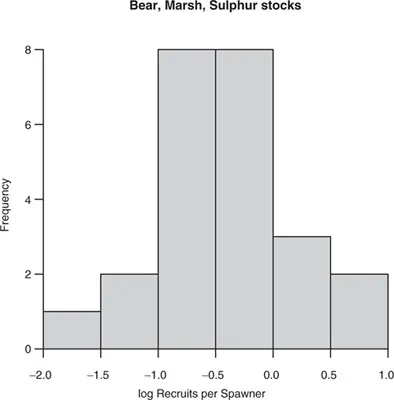
Figure 1.3 Frequency distribution of recruits per spawner for the Bear, Marsh, and Sulphur Creek stocks of spring/summer run Chinook salmon in “good” years.

2. Spawning success E is highly variable (Figure 1.3). In “bad years,” E is essentially nil (about 0.05). About 18% of years (2/11 in the available data) are bad. In “good years,” E can be large or small, and on average it is 0.72 (standard deviation 0.42). What makes years good versus bad may be related to El Niño (Levin et al. 2001).

For this simple illustration, we will ignore the fact that E varies over time and use instead a single “typical” value (in later chapters we discuss models that include variability over time). The median value of E is 0.56 and the average is 0.58, so for the moment let us take E = 0.57. The model is then

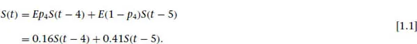
This is the dynamic equation that allows us to predict the future. Current spawners S(t) come from two sources: those offspring of spawners four years ago who return at age four, and those offspring of spawners five years ago who return at age five. The model is nothing more than bookkeeping expressed in mathematical notation. So, to predict the number of spawners in 2002 from data in pre...