Elliptic Tales

Curves, Counting, and Number Theory

Avner Ash, Robert Gross

• Publisher: Princeton University Press
• Year: 2012
• ISBN:
  9781400841714
• Topic: Mathematik
• Subtopic: Geschichte & Philosophie der Mathematik

A look at one of the most exciting unsolved problems in mathematics today Elliptic Tales describes the latest developments in number theory by looking at one of the most exciting unsolved problems in contemporary mathematics—the Birch and Swinnerton-Dyer Conjecture. In this book, Avner Ash and Robert Gross guide readers through the mathematics they need to understand this captivating problem.The key to the conjecture lies in elliptic curves, which may appear simple, but arise from some very deep—and often very mystifying—mathematical ideas. Using only basic algebra and calculus while presenting numerous eye-opening examples, Ash and Gross make these ideas accessible to general readers, and, in the process, venture to the very frontiers of modern mathematics.

PART I

DEGREE

Chapter 1

DEGREE OF A CURVE

Road Map

The idea of degree is a fundamental concept, which will take us several chapters to explore in depth. We begin by explaining what an algebraic curve is, and offer two different definitions of the degree of an algebraic curve. Our job in the next few chapters will be to show that these two different definitions, suitably interpreted, agree.

During our journey of discovery, we will often use elliptic curves as typical examples of algebraic curves. Often, we’ll use y² = x³ − x or y² = x³ + 3x as our examples.

1. Greek Mathematics

In this chapter, we will begin exploring the concept of the degree of an algebraic curve—that is, a curve that can be defined by polynomial equations. We will see that a circle has degree 2. The ancient Greeks also studied lines and planes, which have degree 1. Euclid limited himself to a straightedge and compass, which can create curves only of degrees 1 and 2. A “primer” of these results may be found in the Elements (Euclid, 1956). Because 1 and 2 are the lowest degrees, the Greeks were very successful in this part of algebraic geometry. (Of course, they thought only of geometry, not of algebra.)

Greek mathematicians also invented methods that constructed higher degree curves, and even nonalgebraic curves, such as spirals. (The latter cannot be defined using polynomial equations.) They were aware that these tools enabled them to go beyond what they could do with straight-edge and compass. In particular, they solved the problems of doubling the cube and trisecting angles. Both of these are problems of degree 3, the same degree as the elliptic curves that are the main subject of this book. Doubling the cube requires solving the equation x³ = 2, which is clearly degree 3. Trisecting an angle involves finding the intersection of a circle and a hyperbola, which also turns out to be equivalent to solving an equation of degree 3. See Thomas (1980, pp. 256–261, pp. 352–357, and the footnotes) and Heath (1981, pp. 220–270) for details of these constructions. Squaring the circle is beyond any tool that can construct only algebraic curves; the ultimate reason is that π is not the root of any polynomial with integer coefficients.

Figure 1.1. Three curves

As in the previous two paragraphs, we will see that the degree is a useful way of arranging algebraic and geometric objects in a hierarchy. Often, the degree coincides with the level of difficulty in understanding them.

2. Degree

We have a feeling that some shapes are simpler than others. For example, a line is simpler than a circle, and a circle is simpler than a cubic curve; see figure 1.1

You might argue as to whether a cubic curve is simpler than a sine wave or not. Once algebra has been developed, we can follow the lead of French mathematician René Descartes (1596–1650), and try writing down algebraic equations whose solution sets yield the curves in which we are interested. For example, the line, circle, and cubic curve in figure 1.1 have equations x + y = 0, x² + y² = 1, and y² = x³ − x − 1, respectively. On the other hand, as we will see, the sine curve cannot be described by an algebraic equation.

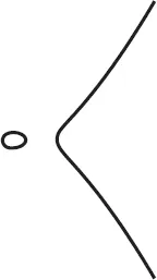
Figure 1.2. y² = x³ − x

Our typical curve with degree 3 has the equation y² = x³ − x. As we can see in figure 1.2, the graph of this equation has two pieces.

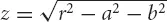
We can extend the concept of equations to higher dimensions also. For example a sphere of radius r can be described by the equation

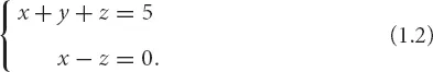
A certain line in 3-dimensional space is described by the pair of simultaneous equations

The “solution set” to a system of simultaneous equations is the set of all ways that we can assign numbers to the variables and make all the equations in the system true at the same time. For example, in the equation of the sphere (which is a “system of simultaneous equations” containing only one equation), the solution set is the set of all triples of the form

This means: To get a single element of the solution set, you pick any two numbers a and b, and you set x = a, y = b, and

or

. (If you don’t want to use complex numbers, and you only want to look at the “real” sphere, then you should make sure that a² + b² ≤ r².)

Similarly, the solution set to the pair of linear equations in (1.2) can be described as the set of all triples

(x, y, z) = (t, 5 − 2t, t),

where t can be any number.

As for our prototypical cubic curve y² = x³ − x, we see that its solution set includes (0, 0), (1, 0), and (−1, 0), but it is difficult to see what the entire set of solutions is.

In this book, we will consider mostly systems of algebraic equations. That means by definition that both sides of th...