Yield Curve Modeling and Forecasting

The Dynamic Nelson-Siegel Approach

Francis X. Diebold, Glenn D. Rudebusch

• Publisher: Princeton University Press
• Year: 2013
• ISBN:
  9781400845415
• Topic: Economics
• Subtopic: Economic Theory
• Index: Economics

Understanding the dynamic evolution of the yield curve is critical to many financial tasks, including pricing financial assets and their derivatives, managing financial risk, allocating portfolios, structuring fiscal debt, conducting monetary policy, and valuing capital goods. Unfortunately, most yield curve models tend to be theoretically rigorous but empirically disappointing, or empirically successful but theoretically lacking. In this book, Francis Diebold and Glenn Rudebusch propose two extensions of the classic yield curve model of Nelson and Siegel that are both theoretically rigorous and empirically successful. The first extension is the dynamic Nelson-Siegel model (DNS), while the second takes this dynamic version and makes it arbitrage-free (AFNS). Diebold and Rudebusch show how these two models are just slightly different implementations of a single unified approach to dynamic yield curve modeling and forecasting. They emphasize both descriptive and efficient-markets aspects, they pay special attention to the links between the yield curve and macroeconomic fundamentals, and they show why DNS and AFNS are likely to remain of lasting appeal even as alternative arbitrage-free models are developed.
Based on the Econometric and Tinbergen Institutes Lectures, Yield Curve Modeling and Forecasting contains essential tools with enhanced utility for academics, central banks, governments, and industry.

1

Facts, Factors, and Questions

In this chapter we introduce some important conceptual, descriptive, and theoretical considerations regarding nominal government bond yield curves. Conceptually, just what is it that are we trying to measure? How can we best understand many bond yields at many maturities over many years? Descriptively, how do yield curves tend to behave? Can we obtain simple yet accurate dynamic characterizations and forecasts? Theoretically, what governs and restricts yield curve shape and evolution? Can we relate yield curves to macroeconomic fundamentals and central bank behavior?

These multifaceted questions are difficult yet very important. Accordingly, a huge and similarly multifaceted literature attempts to address them. Numerous currents and cross-currents, statistical and economic, flow through the literature. There is no simple linear thought progression, self-contained with each step following logically from that before. Instead the literature is more of a tangled web; hence our intention is not to produce a “balanced” survey of yield curve modeling, as it is not clear whether that would be helpful or even what it would mean. On the contrary, in this book we slice through the literature in a calculated way, assembling and elaborating on a very particular approach to yield curve modeling. Our approach is simple yet rigorous, simultaneously in close touch with modern statistical and financial economic thinking, and effective in a variety of situations. But we are getting ahead of ourselves. First we must lay the groundwork.

1.1 Three Interest Rate Curves

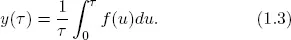
Here we fix ideas, establish notation, and elaborate on key concepts by recalling three key theoretical bond market constructs and the relationships among them: the discount curve, the forward rate curve, and the yield curve. Let P(τ) denote the price of a τ-period discount bond, that is, the present value of $1 receivable τ periods ahead. If y(τ) is its continuously compounded yield to maturity, then by definition

Hence the discount curve and yield curve are immediately and fundamentally related. Knowledge of the discount function lets one calculate the yield curve.

The discount curve and the forward rate curve are similarly fundamentally related. In particular, the forward rate curve is defined as

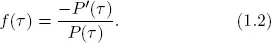
Thus, just as knowledge of the discount function lets one calculate the yield curve, so too does knowledge of the discount function let one calculate the forward rate curve.

Equations (1.1) and (1.2) then imply a relationship between the yield curve and forward rate curve,

In particular, the zero-coupon yield is an equally weighted average of forward rates.

The upshot for our purposes is that, because knowledge of any one of P(τ), y(τ), and f(τ) implies knowledge of the other two, the three are effectively interchangeable. Hence with no loss of generality one can choose to work with P(τ), y(τ), or f(τ). In this book, following much of both academic and industry practice, we work with the yield curve, y(τ). But again, the choice is inconsequential in theory.

Complications arise in practice, however, because although we observe prices of traded bonds with various amounts of time to maturity, we do not directly observe yields, let alone the zero-coupon yields at fixed standardized maturities (e.g., six-month, ten-year, …), with which we work throughout. Hence we now provide some background on yield construction.

1.2 Zero-Coupon Yields

In practice, yield curves are not observed. Instead, they must be estimated from observed bond prices. Two historically popular approaches to constructing yields proceed by fitting a smooth discount curve and then converting to yields at the relevant maturities using formulas (1.2) and (1.3).

The first discount curve approach to yield curve construction is due to McCulloch (1971, 1975), who models the discount curve using polynomial splines.¹ The fitted discount curve, however, diverges at long maturities due to the polynomial structure, and the corresponding yield curve inherits that unfortunate property. Hence such curves can provide poor fits to yields that flatten out with maturity, as emphasized by Shea (1984).

An improved discount curve approach to yield curve construction is due to Vasicek and Fong (1982), who model the discount curve using exponential splines. Their clever use of a negative transformation of maturity, rather than maturity itself, ensures that forward rates and zero-coupon yields converge to a fixed limit as maturity increases. Hence the Vasicek-Fong approach may be more successful at fitting yield curves with flat long ends.

Notwithstanding the progress of Vasicek and Fong (1982), discount curve approaches remain potentially problematic, as the implied forward rates are not necessarily positive. An alternative and popular approach to yield construction is due to Fama and Bliss (1987), who construct yields not from an estimated discount curve, but rather from estimated forward rates at the observed maturities. Their method sequentially constructs the forward rates necessary to price successively longer-maturity bonds. Those forward rates are often called “unsmoothed Fama-Bliss” forward rates, and they are transformed to unsmoothed Fama-Bliss yields by appropriate averaging, using formula (1.3). The unsmoothed Fama-Bliss yields exactly price the included bonds. Unsmoothed Fama-Bliss yields are often the “raw” yields to which researchers fit empirical yield curves, such as members of the Nelson-Siegel family, about which we have much to say throughout this book. Such fitting effectively smooths the unsmoothed Fama-Bliss yields.

1.3 Yield Curve Facts

At any time, dozens of different yields may be observed, corresponding to different bond maturities. But yield curves evolve dynamically; hence they have not only a cross-sectional, but also a temporal, dimension.² In this section we address the obvious descriptive question: How do yields tend to behave across different maturities and over time?

The situation at hand is in a sense very simple—modeling and forecasting a time series—but in another sense rather more complex and interesting, as the series to be modeled is in fact a series of curves.³ In Figure 1.1 we show the resulting three-dimensional surface for the United States, with yields shown as a function of maturity, over time. The figure reveals a key yield curve fact: yield curves move a lot, shifting among different shapes: increasing at increasing or decreasing rates, decreasing at increasing or decreasing rates, flat, U-shaped, and so on.

Table 1.1 presents descriptive statistics for yields at various maturities. Several well-known and important yield curve facts emerge. First, time-averaged yields (the “average yield curve”) increase with maturity; that is, term premia appear to exist, perhaps due to risk aversion, liquidity preferences, or preferred habitats. Second, yield volatilities decrease with maturity, presumably because long rates involve averages of expected future short rates. Third, yields are highly persistent, as evidenced not only by the very large 1-month autocorrelations but also by the sizable 12-month autocorrelations.

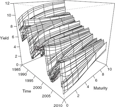
Figure 1.1. Bond Yields in Three Dimensions. We plot end-of-month U.S. Treasury bill and bond yields at maturities ranging from 6 months to 10 years. Data are from the Board of Governors of the Federal Reserve System, based on Gürkaynak et al. (2007). The sample period is January 1985 through December 2008.

Table 1.2 shows the same descriptive statistics for yield spreads relative to the 10-year bond. Yield spread dynamics contrast rather sharply with those of yield levels; in particular, spreads are noticeably less volatile and less persistent. As with yields, the 1-month spread autocorrelations are very large, but they decay more quickly, so that the 12-month spread autocorrelations are noticeably smaller than those for yields. Indeed many strategies for active bond trading (sometimes successful and sometimes not!) are based on spread reversion.

Table 1.1. Bond Yield Statistics

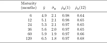
Notes: We present descriptive statistics for end-of-month yields at various maturities. We show sample mean, sample standard deviation, and first- and twelfth-order sample autocorrelations. Data are from the Board of Governors of the Federal Reserve System. The sample period is January 1985 through December 2008.

1.4 Yield Curve Factors

Multivariate models are required for sets of bond yields. An obvious model is a vector autoregression or some close relative. But unrestricted vector autoregressions are profligate parameterizations, wasteful of degrees of freedom. Fortunately, it turns out that financial asset returns typically conform to a certain type of restricted vector autoregression, displaying factor structure. Factor structure is said to be operative in situations where one sees a high-dimensional object (e.g., a large set of bond yields), but where that high-dimensional object is driven by an underlying lower-dimensional set of objects, or “factors.” Thus beneath a high-dimensional seemingly complicated set of observations lies a much simpler reality.

Indeed factor structure is ubiquitous in financial markets, financial economic theory, macroeconomic fundamentals, and macroeconomic theory. Campbell et al. (1997), for example, discuss aspects of empirical factor structure in financial markets and theoretical factor structure in financial economic models.⁴ Similarly, Aruoba and Diebold (2010) discuss empirical factor structure in macroeconomic fundamentals, and Diebold and Rudebusch (1996) discuss theoretical factor structure in macroeconomic models.

Table 1.2. Yield Spread Statistics

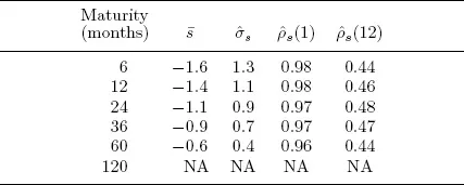
Notes: We present descriptive statistics for end-of-month yield spreads (relative to the 10-year bond) at various maturities. We show sample mean, sample standard deviation, and first- and twelfth-order sample autocorrelations. Data are from the Board of Governors of the Federal Reserve System, based on Gürkaynak et al. (2007). The sample period is January 1985 through December 2008.

In particular, factor structure provides a fine description of the term structure of bond yields.⁵ Most early studies involving mostly long rates implicitly adopt a single-factor world view (e.g., Macaulay (1938)), where the factor is the level (e.g., a long rate). Similarly, early arbitrage-free models like Vasicek (1977) involve only a single factor. But single-factor structure severely limits the scope for interesting term structure dynamics, which rings hollow in terms of both introspection and observation.

Figure 1.2. Bond Yields in Two Dimensions. We plot end-of-month U.S. Treasury bill and bond yields at maturities of 6, 12, 24, 36, 60, and 120 months. Data are from the Board of Governors of the Federal Reserve System, based on Gürkaynak et al. (2007). The sample period is January 1985 through December 2008.

In Figure 1.2 we show a time-series plot of a standard set of bond yields. Clearly they do tend to move noticeably together, but at the same time, it’s clear that more than just a common level factor is operative. In the real world, term structure data—and, correspondingly, modern empirical term structure models—involve multiple factors. This classic recognition traces to Litterman and Scheinkman (1991), Willner (1996), and Bliss ...