Rational Expectations and Inflation

Third Edition

Thomas J. Sargent

• Publisher: Princeton University Press
• Year: 2013
• Print ISBN: 9780691158709
• eBook ISBN: 9781400847648
• Edition: 3
• Topic: Economics
• Subtopic: Banks & Banking
• Index: Economics

A fully expanded edition of the Nobel Prize–winning economist's classic book

This collection of essays uses the lens of rational expectations theory to examine how governments anticipate and plan for inflation, and provides insight into the pioneering research for which Thomas Sargent was awarded the 2011 Nobel Prize in economics. Rational expectations theory is based on the simple premise that people will use all the information available to them in making economic decisions, yet applying the theory to macroeconomics and econometrics is technically demanding. Here, Sargent engages with practical problems in economics in a less formal, noneconometric way, demonstrating how rational expectations can satisfactorily interpret a range of historical and contemporary events. He focuses on periods of actual or threatened depreciation in the value of a nation's currency. Drawing on historical attempts to counter inflation, from the French Revolution and the aftermath of World War I to the economic policies of Margaret Thatcher and Ronald Reagan, Sargent finds that there is no purely monetary cure for inflation; rather, monetary and fiscal policies must be coordinated.

This fully expanded edition of Rational Expectations and Inflation includes Sargent's 2011 Nobel lecture, "United States Then, Europe Now." It also features new articles on the macroeconomics of the French Revolution and government budget deficits.

1

Rational Expectations and the
Reconstruction of Macroeconomics

The government has strategies. The people have counterstrategies.

Ancient Chinese proverb

Behavior Changes with the Rules of the Game

In order to provide quantitative advice about the effects of alternative economic policies, economists have constructed collections of equations known as econometric models.¹ For the most part these models consist of equations that attempt to describe the behavior of economic agents—firms, consumers, and governments—in terms of variables that are assumed to be closely related to their situations. Such equations are often called decision rules because they describe the decisions people make about things like consumption rates, investment rates, and portfolios as functions of variables that summarize the information people use to make those decisions. For all of their mathematical sophistication, econometric models amount to statistical devices for organizing and detecting patterns in the past behavior of people’s decision making, patterns that can then be used as a basis for predicting their future behavior.

As devices for extrapolating future behavior from the past under a given set of rules of the game, or government policies, these models appear to have performed well.² They have not performed well, however, when the rules changed. In formulating advice for policymakers, economists have routinely used these models to predict the consequences of historically unprecedented, hypothetical government interventions that can only be described as changes in the rules of the game. In effect, the models have been manipulated in a way that amounts to assuming that people’s patterns of behavior do not depend on those properties of the environment that government interventions would change. The assumption has been that people will act under the new rules just as they have under the old, so that even under new rules, past behavior is still a reliable guide to future behavior. Econometric models used in this way have not been able to predict accurately the consequences of historically unparalleled interventions.³ To take one recent example, standard Keynesian and monetarist econometric models built in the last 1960s failed to predict the effects on output, employment, and prices that were associated with the unprecedented large deficits and rates of money creation of the 1970s.

Recent research has been directed at building econometric models that take into account that people’s behavior patterns will vary systematically with changes in government policies—the rules of the game.⁴ Most of this research has been conducted by adherents of the so-called hypothesis of rational expectations. They model people as making decisions in dynamic settings in the face of well-defined constraints. Included among these constraints are laws of motion over time that describe such things as the taxes people must pay and the prices of the goods they buy and sell. The hypothesis of rational expectations is that people understand these laws of motion. The aim of the research is to build models that can predict how people’s behavior will change when they are confronted with well-understood changes in ways of administering taxes, government purchases, aspects of monetary policy, and the like.

THE INVESTMENT DECISION

A simple example will illustrate both the principle that decision rules depend on the laws of motion that agents face and the extent that standard macroeconomics models have violated this principle. Let k_t be the capital stock of an industry and τ_t be a tax rate on capital. Let τ_t be the first element of z_t, a vector of current and lagged variables, including those that the government considers when it sets the tax rate on capital. We have τ_t ≡ e^Tz_t, where e is the unit vector with unity in the first place and zeros elsewhere.⁵ Let a firm’s optimal accumulation plan require that capital acquisitions obey⁶

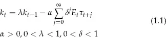
where E_tτ_t+j is the tax rate at time t that is expected to prevail at time t + j.

Equation 1.1 captures the notion that the demand for capital responds negatively to current and future tax rates. However, equation 1.1 does not become an operational investment schedule or decision rule until we specify how agents’ views about the future, E_tτ_t+j, are formed. Let us suppose that the actual law of motion for z_t is

where A is a matrix conformable with z_t.⁷ If agents understand this law of motion for z_t, the first element of which is τ_t, then their best forecast of τ_t+j is e^T A^jz_t. We impose rational expectations by equating agents’ expectations E_tτ_t+j to this best forecast. Upon imposing rational expectations, some algebraic manipulation implies the operational investment schedule

In terms of the list of variables on the right-hand side, equation (1.3) resembles versions of investment schedules that were fit in the heyday of Keynesian macroeconomics in the 1960s. This is not unusual, for the innovation of rational expectations reasoning is much more in the ways equations are interpreted and manipulated to make statements about economic policy than in the look of the equations that are fit. Indeed, the similarity of standard and rational expectations equations suggests what can be shown to be true generally: The rational expectations reconstruction of macroeconomics is not mainly directed at improving the statistical fits of Keynesian or monetarist macroeconomics models over given historical periods and that its success or failure cannot be judged by comparing the R^2’s of reconstructed macroeconomics models with those of models constructed and interpreted along earlier lines.

Under the rational expectations assumption, the investment schedule (equation (1.3)) and the laws of motion for the tax rate and the variables that help predict it (equation (1.2)) have a common set of parameters, namely, those of the matrix A. These parameters appear in the investment schedule because they influence agents’ expectations of how future tax rates will affect capital. Further, notice that all of the variables in z_t appear in the investment schedule, since via equation (1.2) all of these variables help agents forecast future tax rates. (Compare this with the common econometric practice of using only current and lagged values of the tax rate as proxies for expected future tax rates.)

The fact that equations (1.2) and (1.3) share a common set of parameters (the A matrix) reflects the principle that firms’ optimal decision rule for accumulating capital, described as a function of current and lagged state and information variables, will depend on the constraints (or laws of motion) that firms face. That is, the firm’s pattern of investment behavior will respond systematically to the rules of the game for setting the tax rate τ_t. A widely understood change in the policy for administering the tax rate can be represented as a change in the first row of the A matrix. Any such change in the tax rate regime or policy will thus result in a change in the investment schedule (equation (1.3)). The dependence of the coefficients of the investment schedule on the environmental parameters in matrix A is reasonable and readily explicable as a reflection of the principle that agents’ rules of behavior change when they encounter changes in the environment in the form of new laws of motion for variables that constrain them.

To illustrate this point, consider two specific tax rate policies. First, consider the policy of a constant tax rate τ_t+j = τ_t for all j ≥ 0. Then z_t = τ₁, A = 1, and the investment schedule is

where h₀ = –α/(1 + δ). Now consider an investment tax credit on-again, off-again tax rate policy of the form τ_t = – τ_t–1. In this case z_t = τ₁, A = –1, and the investment schedule becomes

where h₀ = –α/(1 + δ). Here the investment schedule itself changes as the policy for setting the tax rate changes.

Standard econometric practice has not acknowledged that this sort of thing happens. Returning to the more general investment example, the usual econometric practice has been roughly as follows. First, a model is typically specified and estimated of the form

where h is a vector of free parameters of dimension conformable with the vector z_t. Second, holding the parameters h fixed, equation (1.6) is used to predict the implications of alternative paths for the tax rate τ_t. This procedure is equivalent to estimating equation (1.4) from historical data when τ_t = τ_t–1 and then using this same equation to predict the consequences for capital accumulation of instituting an on-again, off-again tax rate policy of the form τ_t = –τ_t–1. Doing this assumes that a single investment schedule of the form of equation (1.6) can be found with a single parameter vector h that will remain fixed regardless of the rules for administering the tax rate.⁸

The fact that equations (1.2) and (1.3) share a common set of parameters implies that the search for such a regime-independent decision schedul...

Table of contents

• Cover Page
• Title Page
• Copyright Page
• Dedication Page
• Contents
• List of Figures
• List of Tables
• Acknowledgements
• Preface to the Third Edition
• Preface to the Second Edition
• Preface to the First Edition
• 1. Rational Expectations and the Reconstruction of Macroeconomics
• 2. Reaganomics and Credibility
• 3. The Ends of Four Big Inflations
• 4. Stopping Moderate Inflations: the Methods of Poincaré and Thatcher
• 5. Some Unpleasant Monetarist Arithmetic
• 6. Interpreting the Reagan Deficits
• 7. Speculations About the Speculation Against the Hong Kong Dollar
• 8. Six Essays in Persuasion
• 9. Macroeconomic Features of the French Revolution
• 10. United States Then, Europe Now
• References
• Author Index
• Subject Index