Bayesian Non- and Semi-parametric Methods and Applications

Peter Rossi

• Publisher: Princeton University Press
• Year: 2014
• Print ISBN: 9780691145327
• eBook ISBN: 9781400850303
• Topic: Economics
• Subtopic: Economic Theory
• Index: Economics

This book reviews and develops Bayesian non-parametric and semi-parametric methods for applications in microeconometrics and quantitative marketing. Most econometric models used in microeconomics and marketing applications involve arbitrary distributional assumptions. As more data becomes available, a natural desire to provide methods that relax these assumptions arises. Peter Rossi advocates a Bayesian approach in which specific distributional assumptions are replaced with more flexible distributions based on mixtures of normals. The Bayesian approach can use either a large but fixed number of normal components in the mixture or an infinite number bounded only by the sample size. By using flexible distributional approximations instead of fixed parametric models, the Bayesian approach can reap the advantages of an efficient method that models all of the structure in the data while retaining desirable smoothing properties. Non-Bayesian non-parametric methods often require additional ad hoc rules to avoid "overfitting," in which resulting density approximates are nonsmooth. With proper priors, the Bayesian approach largely avoids overfitting, while retaining flexibility. This book provides methods for assessing informative priors that require only simple data normalizations. The book also applies the mixture of the normals approximation method to a number of important models in microeconometrics and marketing, including the non-parametric and semi-parametric regression models, instrumental variables problems, and models of heterogeneity. In addition, the author has written a free online software package in R, "bayesm," which implements all of the non-parametric models discussed in the book.

1

Mixtures of Normals

In this chapter, I will review the mixture of normals model and discuss various methods for inference with special attention to Bayesian methods. The focus is entirely on the use of mixtures of normals to approximate possibly very high dimensional densities. Prior specification and prior sensitivity are important aspects of Bayesian inference and I will discuss how prior specification can be important in the mixture of normals model. Examples from univariate to high dimensional will be used to illustrate the flexibility of the mixture of normals model as well as the power of the Bayesian approach to inference for the mixture of normals model. Comparisons will be made to other density approximation methods such as kernel density smoothing which are popular in the econometrics literature.

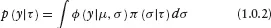
The most general case of the mixture of normals model “mixes” or averages the normal distribution over a mixing distribution.

Here π( ) is the mixing distribution. π( ) can be discrete or continuous. In the case of univariate normal mixtures, an important example of a continuous mixture is the scale mixture of normals.

A scale mixture of a normal distribution simply alters the tail behavior of the distribution while leaving the resultant distribution symmetric. Classic examples include the t distribution and double exponential in which the mixing distributions are inverse gamma and exponential, respectively (Andrews and Mallows (1974)). For our purposes, we desire a more general form of mixing which allows the resultant mixture distribution sufficient flexibility to approximate any continuous distribution to some desired degree of accuracy. Scale mixtures do not have sufficient flexibility to capture distributions that depart from normality exhibiting multi-modality and skewness. It is also well-known that most scale mixtures that achieve thick tailed distributions such as the Cauchy or low degree of freedom t distributions also have rather “peaked” densities around the mode of the distribution. It is common to find datasets where the tail behavior is thicker than the normal but the mass of the distribution is concentrated near the mode but with rather broad shoulders (e.g., Tukey’s “slash” distribution). Common scale mixtures cannot exhibit this sort of behavior. Most importantly, the scale mixture ideas do not easily translate into the multivariate setting in that there are few distributions on Σ for which analytical results are available (principally the Inverted Wishart distribution).

For these reasons, I will concentrate on finite mixtures of normals. For a finite mixture of normals, the mixing distribution is a discrete distribution which puts mass on K distinct values of μ and Σ.

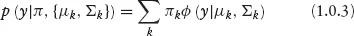
ϕ( ) is the multivariate normal density.

d is the dimension of the data, y. The K mass points of the finite mixture of normals are often called the components of the mixture. The mixture of normals model is very attractive for two reasons: (1) the model applies equally well to univariate and multivariate settings; and (2) the mixture of normals model can achieve great flexibility with only a few components.

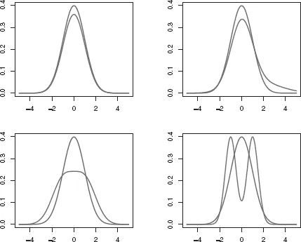
Figure 1.1. Mixtures of Univariate Normals

Figure 1.1 illustrates the flexibility of the mixture of normals model for univariate distributions. The upper left corner of the figure displays a mixture of a standard normal with a normal with the same mean but 100 times the variance (the red density curve), that is the mixture .95N(0, 1) + .05N(0, 100). This mixture model is often used in the statistics literature as a model for outlying observations. Mixtures of normals can also be used to create a skewed distribution by using a “base” normal with another normal that is translated to the right or left depending on the direction of the desired skewness.

The upper right panel of Figure 1.1 displays the mixture, .75N(0, 1) + .25N(1.5, 2²). This example of constructing a skewed distribution illustrates that mixtures of normals do not have to exhibit “separation” or bimodality. If we position a number of mixture components close together and assign each component similar probabilities, then we can create a mixture distribution with a density that has broad shoulders of the type displayed in many datasets. The lower left panel of Figure 1.1 shows the mixture .5N(−1, 1) + .5N(1, 1), a distribution that is more or less uniform near the mode. Finally, it is obvious that we can produce multi-modal distributions simply by allocating one component to each desired model. The bottom right panel of the figure shows the mixture .5N(−1, .5²) + .5N(1, .5²). The darker lines in Figure 1.1 show a unit normal density for comparison purposes.

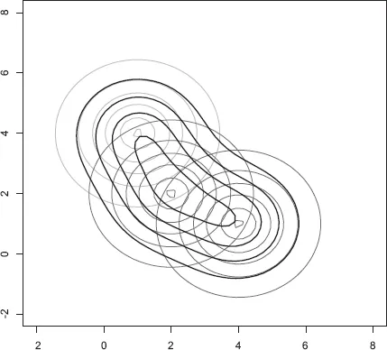
Figure 1.2. A Mixture of Bivariate Normals

In the multivariate case, the possibilities are even broader. For example, we could approximate a bivariate density whose contours are deformed ellipses by positioning two or more bivariate normal mixtures along the principal axis of symmetry. The “axis” of symmetry can be a curve allowing for the creation of a density with “banana” or any other shaped contour. Figure 1.2 shows a mixture of three uncorrelated bivariate normals that have been positioned to obtain “bent” or “banana-shaped” contours.

There is an obvious sense in which the mixture of normals approach, given enough components, can approximate any multivariate density (see Ghosh and Ramamoorthi (2003) for infinite mixtures and Norets and Pelenis (2011) for finite mixtures). As long as the density which is approximated by the mixture of normals damps down to zero before reaching the boundary of the set on which the density is defined, then mixture of normals models can approximate the density. Distributions (such as truncated distributions) with densities that are non-zero at the boundary of the sample space will be problematic for normal mixtures. The intuition for this result is that if we were to use extremely small variance normal components and position these as needed in the support of the density then any density can be approximated to an arbitrary degree of precision with enough normal components. As long as arbitrarily large samples are allowed, then we can afford a larger and larger number of these tiny normal components. However, this is a profligate and very inefficient use of model parameters. The resulting approximations, for any given sample size, can be very non-smooth, particularly if non-Bayesian methods are used. For this reason, the really interesting question is not whether the mixture of normals can be the basis of a non-parametric density estimation procedure, but, rather, if good approximations can be achieved with relative parsimony. Of course, the success of the mixture of normals model in achieving the goal of flexible and relatively parsimonious approximations will depend on the nature of the distributions that need to be approximated. Distributions with densities that are very non-smooth and have tremendous integrated curvature (i.e., lots of wiggles) may require large numbers of normal components.

The success of normal mixture models is also tied to the methods of inference. Given that many multivariate density approximation situations will require a reasonably large number of components and each component will have a very large number of parameters, inference methods that can handle very high dimensional spaces will be required. Moreover, the inference methods that over-fit the data will be particularly problematic for normal mixture models. If an inference procedure is not prone to over-fitting, then inference can be conducted for models with a very large number of components. This will effectively achieve the non-parametric goal of sufficient flexibility without delivering unreasonable estimates. However, an inference method that has no method of curbing over-fitting will have to be modified to penalize for over-parameterized models. This will add another burden to the user—choice and tuning of a penalty function.

1.1 Finite Mixture of Normals Likelihood Function

There are two alternative ways of expressing the likelihood function for the mixture of normals model. This first is s...

Table of contents

• Cover Page
• Title Page
• Copyright Page
• Contents
• Preface
• 1 Mixtures of Normals
• 2 Dirichlet Process Prior and Density Estimation
• 3 Non-parametric Regression
• 4 Semi-parametric Approaches
• 5 Random Coefficient Models
• 6 Conclusions and Directions for Future Research
• Bibliography
• Index