Tools and Techniques for Financial Stability Analysis

Indranarain Ramlall

• Publisher: Emerald Publishing Limited
• Year: 2018
• ISBN:
  9781787568471
• Topic: Business
• Subtopic: Finance
• Index: Business

Combatting financial stability risks is a highly challenging task which can by no means be concentrated into a 'one-size fits all' approach. It is important to select the appropriate tools and techniques in order to monitor, analyse, and maintain financial stability through proactive policy measures.
Tools and Techniques for Financial Stability Analysis explores all key aspects of analytical tools and challenges for sound financial stability assessments. Comprehensive coverage is given to value at risk, stress testing, graphical tools for financial stability, the financial system stress index, as well as ratios and metrics of financial stability assessment. Finally, a concluding chapter is devoted to understand the key challenges involved in maintaining financial stability.
This book will prove valuable to central bankers, economists, and policy-makers who are involved in the field of financial stability, as well as researchers studying the field.

Chapter 1

Value at Risk

1.1. Definition of Value at Risk

Value at risk (VaR) can be succinctly defined as the maximum level of loss which can be borne by an institution at a given time period over a specified confidence level. Compared to other forms of risk management metrics, the VaR risk indicator represents a form of downside risk. Technically speaking, the VaR for t days is calculated as the VaR for one day multiplied by the square root of time. The statistical value for 95%, 99% and 99.5% in the case of VaR is 1.645, 2.326 and 2.58, respectively. Choosing a high probability, say 99%, signifies that losses higher than the VaR can be tolerated only infrequently. The main assumption of VaR is that the data used are normally distributed which is unlikely to hold true in practice. For instance, financial returns are leptokurtic in nature with exhibition of fat tails. The VaR was particularly useful for the banking sector as it helped in computing the level of capital required to absorb feasible unexpected losses. The selection of the time horizon and the significance level will be a function of the organisation’s ability and willingness to bear the risk.

1.2. Benefits of Var

The VaR is widely used in financial institutions for risk assessment, risk-based capital controls and risk-adjusted performance measurement. The VaR aggregates risk into a single component. VaR can be applied to different types of risks to thereby constitute a metric which enables comparative assessments of the distinct types of risks which buffet any institution. VaR gained prominence in the world on the back of being easy to apply and to understand. VaR is able to capture the level of risk aversion through the confidence level. As a matter of fact, the choice of the confidence level in VaR should sieve out the risk aversion level of the company. Thus, a higher level of risk aversion is reflected through a higher confidence level or a lower significance level which is also same as a higher statistical value of VaR.

1.3. Limitations of Var

No metric of risk assessment is fully perfect and so is the case for VaR. The VaR has certain limitations such as overlooking of the upside potential, being good only to the extent that the inputs used are good and relying on normality assumptions.

In relation to financial stability, VaR has not been a good student. This can best be captured by Choudhry (2013) who comments that VaR underestimates risks during the Great Recession, a time when it was most needed, belittling the robustness of VaR as a reliable risk management tool. This induced the Basel Committee on Banking Supervision to scrap VaR in favour of Expected Shortfall (ES). In contrast to VaR which gauges on ‘How bad can things get?’, ES asks the question ‘If things get bad, what is our expected loss?’. In essence, ES calculates the expected value of losses beyond a stated confidence level.

The VaR suffers from non-additive principle, that is, the VaR of a portfolio of two assets is not the same as the combined sum of VaRs of these two assets individually, signifying the need to give due consideration to correlation whenever focusing on portfolio VaR.

The VaR fails to sieve out the true value of loss in the case that strong fat tails permeate the data-generating process of the asset under scrutiny which thereby infringes the assumption of normality. Recourse can be made to the Student t-distribution of the generalised hyperbolic distribution (GHD) to deal with such a problem. In a parallel manner, the non-stationarity principle represents a statistical warning that the past is not necessarily a guide to the future. Under extreme economic situations, historical relationships easily break apart.

Illiquidity: if securities do not trade in highly liquid markets, reliable prices are not available to compute rates of return. Alarmingly, if there are large adverse price movements, portfolio managers may not be able to dispose of large quantities of the security without unleashing a fall in the share price, particularly if other portfolio managers are doing the same. The VaR will underestimate the severity of bad outcomes unless markets are highly liquid.

Non-linearity: standard VaR calculations do not allow for non-linear relationships. For example, a 2% change in the security price may cause the portfolio to lose US$1million but a 4% change may generate it to lose US$10million. Non-linearities can be accommodated but only at the expense of more risk in the economic model.

Whether the variance-covariance, historical or Monte Carlo approaches are used, all of them assume that the future will repeat itself. This explains the rationale as to why stress testing is deemed to be better than VaR as it is more flexible in incorporating more realistic scenarios. In fact, based on the shortcomings of VaR, it should be complemented with other risk management tools such as stress testing. This is supported by the notion that VaR tends to be rigid in nature because it is based on normal conditions, let alone the fact that it does not factor in what-if conditions.

Despite the abovementioned limitations, yet, VaR is important for risk management. The VaR is often accompanied by stress testing and scenario analysis because VaR is seldom used in isolation.

1.4. Framework Under Var

1.4.1. Distinction between CDF and PDF

Prior to gaining insight on the framework embedded in VaR, it is of paramount significance to master two key tools in statistics, namely the probability density function (PDF) and the cumulative density function (CDF).

1.4.2. Probability Density Function

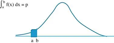
For a continuous random variable X, the PDF can be defined as the probability of outcomes manifesting between any two points. Given a random variable X, the PDF f(x) can be defined as the probability p that X lies in between point a and point b (Figure 1.1).

Figure 1.1. Probability and Cumulative Density Functions. Source: Author’s illustration, x-axis: x; y-axis: f(x).

1.4.3. Cumulative Density Function

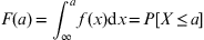
The CDF tells us the probability of a random variable being less than a specific value. Technically speaking, the CDF can be ejected out by integrating the PDF. Hence, differentiating the CDF leads to the PDF. Hence, CDF is read on the same PDF graph but taken as the integral of PDF or area under the curve. In that respect, since probability can never exceed one and never be negative, the value of CDF ranges from zero to one.

Conventionally, the CDF is denoted by capital letters. Hence, for a random variable X with a PDF f(x), the CDF is F(x).

1.5. The Generalised Hyperbolic Distribution

Returns from financial variables like stock prices, interest rates and exchange rates are usually characterised by more peakedness and heavy tails than normal distribution. The GHD was introduced by Barndorff-Nielsen (1977) who introduced GHDs in the study of grains of sand. Since its development, the GHD has been applied in diverse fields like physics, bio...