![]()
1
CHARACTERIZATION OF SEMICONDUCTOR NANOSTRUCTURES BY SCANNING ELECTRON MICROSCOPY
Lynne M. Gignac and Oliver C. Wells
IBM T. J. Watson Research Center
Yorktown Heights, NY 10598, USA
__________
1.1. Introduction
1.2. SEM Instrumentation
1.2.1. Electron Sources
1.2.2. Electron Lenses
1.2.3. Electron Detectors
1.2.4. Beam Deceleration/Sample Bias
1.2.5. Aberration Correction
1.2.6. Focused Ion Beam Systems
1.3. Practical Examples
1.3.1. Imaging with Low Incident Beam Energy
1.3.2. Electron Beam Induced Sample Damage
1.3.3. Use of Sample Bias/Beam Deceleration
1.3.4. Use of a Source Monochromator
1.3.5. Secondary Electron Detectors
1.3.6. Use of STEM Detector
1.3.7. Imaging with High Incident Beam Energy
1.4. Conclusions
References
List of Symbols and Acronyms
3-D | = three-dimensional |
α | = aperture or convergence angle |
β | = beam brightness = beam current per unit area per solid angle |
κ | = dielectric constant |
λ | = electron wave length |
θ | = collection scattering angle |
B | = incident electron beam |
BD | = beam deceleration |
BF | = bright field |
BSE | = backscattered electron |
Cc | = chromatic aberration coefficient |
CFE | = cold field emission |
CNT | = carbon nanotube |
Cs | = spherical aberration coefficient |
d1 | = electron beam size or diameter at Wehnelt cylinder |
dg | = demagnified electron beam size |
do | = electron beam size or diameter on sample surface |
DB-FIB | = dual beam focused ion beam |
DF | = dark field |
DoF | = depth of field |
Eo | = incident electron beam energy |
ΔEo | = electron beam energy spread |
EBSP | = electron backscatter patterning |
EDS | = energy dispersive x-ray spectroscopy |
ETD | = Everhart-Thornley detector |
FE | = field emission |
FIB | = focused ion beam |
HAADF | = high angle annular dark field |
i | = beam current |
k | = immersion ratio = Eo/LE |
LE | = landing energy |
LEEM | = low energy electron microscope |
MFP | = mean free path |
PM | = photomultiplier |
SB | = sample bias |
SB-FIB | = single beam focused ion beam |
SE | = secondary electrons |
SEM | = scanning electron microscope |
SE-I | = secondary electrons produced from the incident electron beam |
SE-II | = secondary electrons produced from backscattered electrons |
SE-III | = secondary electrons produced from backscattered electrons hitting components in the microscope (chamber walls, pole piece, etc) |
SFE | = Schottky field emission |
s-MC | = source monochromator |
STEM | = scanning transmission electron microscope |
TEM | = transmission electron microscope |
TTL | = through the lens |
TTLD | = through the lens detector |
Z | = atomic number |
1.1. INTRODUCTION
Nanotechnology is broadly defined as the study of controlling matter on the atomic or molecular size scale, but often the size of structures studied is 10–100 nm. The ability to image tiny, nm-sized structures is vital to most nanotechnology research and development programs. The scanning electron microscope (SEM) has emerged as the work horse imaging tool for nanotechnology studies since it has nanometer scale image resolution, is surface sensitive, and is often relatively easy to use. As semiconductor and nanotechnology fields have advanced and structures have shrunk over the past 20 years, the SEM resolution and capabilities have also improved. Most high performance SEMs have a resolution specification of ~1 nm at an incident electron beam energy (Eo) of 15keV. A modern transmission electron microscope (TEM) typically has better resolution (e.g. sub-0.1 nm resolution at Eo of 200 keV) and better contrast than a high resolution SEM so there is often a need to image nanostructures using TEM. However, a roadblock for TEM analysis is often the preparation of sub-100 nm thick TEM samples that allows transmission of the electron beam through the sample to produce images with good resolution and contrast. TEM sample preparation can be time consuming and requires great skill, particularly when nanostructures are in the 10s of nm size range. SEM samples often require little or no sample preparation and rapid feedback on nanostructure processing can be obtained when proper resources such as SEM instrumentation and trained operators are available. SEM analysis has become invaluable to the success of a nanotechnology project.
In the first section of this chapter, SEM instrumentation will be reviewed. Since there are already many books devoted to the SEM1–3 and a book devoted to scanning microscopy for nanotechnology,4 this section of the chapter will provide a broad overview of SEM instrumentation, focusing on advances in electron sources, lenses, and detectors that have allowed improved imaging performance. The employment of electron beam deceleration and lens aberration correction also will be discussed. In the second section, practical examples of imaging nanotechnology structures using SEM will be given. From these examples, the reader will see how varying the imaging conditions and detector signals can result in different information about the sample. Knowledge of the benefits of these approaches can give an analyst numerous options to better understand and characterize a sample.
1.2. SEM INSTRUMENTATION
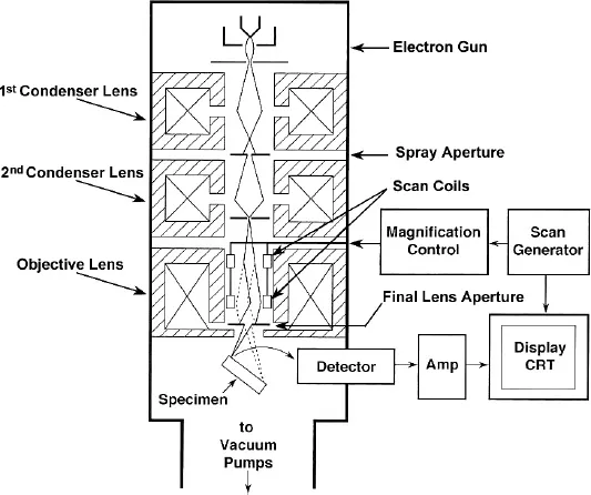
The scanning electron microscope consists of a beam of electrons (B) emitted from a source or gun which is accelerated down a column, and then focused and scanned on a specimen surface. Figure 1.1 shows a schematic diagram of a typical SEM system. Electrons that are produced by the interaction of the incident beam with the atoms in the sample surface are emitted from the sample and detected to form an image. Two types of electrons can be detected in an SEM: secondary (SE) and backscattered (BSE). SE are low energy electrons produced by inelastic collisions of the B and the BSE with sample atoms. BSE are incident beam electrons that elastically scatter at high angles with the nucleus of the sample atoms and are emitted back into the vacuum. SE and BSE will be discussed in more detail in Sec. 1.2.3. Since the emitted electrons are generated from the near surface region, SEM images typically depict the surface structure of the sample and can show the 3-dimensional (3-D) surface variations. The resolution of the image is determined by the size of the interaction volume that the incident beam produces in the sample and the available contrast differences of the materials or surface features being detected.5 The interaction volume is dependent on the electron beam size (do) on the sample surface, incident beam energy (Eo) and specimen material composition.
Fig. 1.1 Schematic diagram of a scanning electron microscope (SEM) system from Ref. 3.
Image resolution is often a difficult parameter to measure for any particular sample so the resolution of the SEM is typically measured on a standard sample consisting of using Au particles on a carbon background.5 The large atomic number (Z) differences in the standard sample allow optimal resolution measurement but this number may not be an accurate measure of the resolution that is obtained for samples studied in any particular lab. As of 2010 most SEM instrument vendors offer instruments with 1 nm resolution at Eo = 15 keV and some vendors offer sub-1 nm resolution at Eo = 1keV.
Over the past 20 years, SEM instrumentation has undergone constant improvements which have been driven by customer needs in both the physical sciences and biological/medical fields to image sample surfaces with better resolution at lower Eo.6,7 The instrumentation improvements can be broken down into several categories: electron sources, lens systems, detectors, beam deceleration, and aberration correction. The following sections will first introduce these features and then discuss how improvements in each feature have helped to advance SEM performance an...