Modeling And Pricing In Financial Markets For Weather Derivatives

Fred Espen Benth, Jūratė Šaltytė Benth

• Publisher: WSPC
• Year: 2012
• Print ISBN: 9789814401845
• eBook ISBN: 9789814401869
• Topic: Biological Sciences
• Subtopic: Science General
• Index: Biological Sciences

Weather derivatives provide a tool for weather risk management, and the markets for these exotic financial products are gradually emerging in size and importance. This unique monograph presents a unified approach to the modeling and analysis of such weather derivatives, including financial contracts on temperature, wind and rain. Based on a deep statistical analysis of weather factors, sophisticated stochastic processes are introduced modeling the time and space dynamics. Applying ideas from the modern theory of mathematical finance, weather derivatives are priced, and questions of hedging analyzed. The treatise contains an in-depth analysis of typical weather contracts traded at the Chicago Mercantile Exchange (CME), including so-called CDD and HDD futures. The statistical analysis of weather variables is based on a large data set from Lithuania.

The monograph includes the research done by the authors over the last decade on weather markets. Their work has gained considerable attention, and has been applied in many contexts.

Contents:

• • Financial Markets for Weather
• Statistics of Weather:
  • Data Description and Exploratory Analysis
  • Spatial-Temporal Modelling
• Weather Derivatives:
  • Continuous-Time Models for Temperature and Wind Speed
  • Pricing of Forward Contracts on Temperature and Wind Speed
  • Extensions of Temperature and Wind Speed Models
  • Options on Temperature and Wind
  • Precipitation Derivatives
  • Utility-Based Approaches to Pricing Weather Derivatives

Readership: Researchers in mathematical/quantitative finance, environmental/energy economics.

Chapter 1

Financial markets for weather

By the year 2011, the notional value of the market for weather derivatives was USD11.8 billion, according to the Weather Risk Management Association (WRMA)¹. The weather markets have grown remarkably in financial strength since the first known weather deals took place in 1996. Nowadays, these markets provide a platform for managing risk exposure in weather variables like temperature, wind and precipitation. The most liquid weather derivatives are based on temperature. In short, these derivatives convert weather into money, where you can profit on bad weather (or good, for that matter).

In this monograph we analyze typical weather derivatives traded in the market, both over-the-counter and as customary assets on exchanges. Our aim is to present a unified approach to the statistical modelling of weather factors like temperature, wind speed and precipitation, and apply these models along with the arbitrage theory of mathematical finance to price weather derivatives. In this first Chapter we present typical weather derivatives and the markets they are traded in, before we move on with the statistical analysis of weather and the pricing of weather derivatives.

1.1 The use of weather derivatives

A skiing resort in the Alps is dependent on snow to operate and profit from tourism. A farmer needs fair weather when harvesting the crop in the autumn. A power producer earns money when the weather is hot and air-conditioning is required. A wind mill farm can only operate when there is wind. If weather conditions are unfavourable, on the other hand, the ski resort will not attract any tourists, the farmer risks to lose the harvest, the wind mill cannot operate or the demand for power may be low. Too cold or too hot temperatures, no wind or too strong wind, drought or flooding, may seriously harm industry and constitute a major risk to revenues. Weather derivatives are designed to offer a financial tool for hedging this risk.

---

¹see www.wrma.org

A farmer, say, can insure the crop against flooding in the harvest season. If there is a flooding, the farmer can claim coverage of the incurred losses based on the insurance contract. However, to make these claims, the farmer must prove that losses are due to the flooding, and this may not be a simple task since also other factors influence the harvest, making it difficult to assess the damage. Weather derivatives, like, for example, derivatives written on rainfall, are an alternative that provides an “objective” way to insure against flooding. Typically, a rainfall derivative is a financial contract that pays the owner money according to an index measuring the amount of rain over a period. For example, the farmer may buy such a contract written on the amount of rain during the harvest season. If there is flooding, the amount of rain will be above a certain threshold, and the contract, properly designed, will pay out money in such a case. The farmer will receive cash, no matter what the actual losses are. The farmer has in effect an insurance against flooding without having to prove any damages. In fact, the farmer will receive money no matter if there is a flooding or not. Of course, the rainfall derivative contract will cost money, which is paid up front at entry.

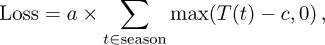
The profit from a skiing resort is directly linked to the weather during the season. Too warm temperatures destroy snow conditions and harm the profit. To make matters simple, let us suppose that the resort can measure the losses being proportional to the aggregate temperatures T(t), with t being time, above a threshold c in the season, that is,

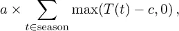
for some proportionality constant a > 0. It is natural to suppose that the threshold c could be equal to, or be slightly above 0 degrees Celsius (°C). The losses will then be proportional to the number of cooling-degree days in the season (see below). Imagine now a temperature derivatives contract which pays the buyer the number of cooling degree days with threshold c over the season measured at the ski resort, in return of a fixed amount F. This would in effect be a futures contract on the cooling-degree day index over the season. The ski resort could buy a such contracts, and would in this case receive

which covers the temperature-dependent losses. On the other hand, the ski resort must pay the amount F. The temperature derivatives contract has in effect swapped their stochastically floating loss function with a fixed one.

Consider now the electricity market, for example, in Southern Europe. It is natural to imagine that the profits of a power producer are proportional to temperatures in the summer due to the demand of air-conditioning cooling. The lower temperature, the lower demand and thus less production of power that leads to reduced income. At the same time, prices of power are likely to go down with lower temperatures. The producer can hedge the production by, for example, selling futures contracts on the cumulative temperature in the summer period, which would generate a fixed income of money (being the futures price) in return of paying the realized cumulative temperature. If this becomes lower than the futures price, the producer generates an income that could cover the losses. On the other hand, the producer will lose on the futures contract if temperatures become high, but in this case generate income from production. In any case, the producer has locked in the loss generated by temperature to be the fixed futures price, and not the random cumulative temperature.

A retailer in the same market typically have fixed price and volume contracts with the clients, and buys power in the market to honour these. As volume increases with increasing temperatures, the retailer may suffer losses incurred by increasing power prices. The retailer may be interested in off-loading the temperature risk by entering long positions in cumulative average temperature futures. A long position in the futures corresponds to buying it, and the retailer will receive the realized cumulative average temperature in return of the fixed futures price. As the retailer on the other hand “pays” the cumulative temperature indirectly in terms of losses, such an investment will make the retailer immune against variations in cumulative temperature. As we see from these two examples, the needs of hedging against temperatures may be opposite for actors in the energy market.

Weather derivatives may prove fruitful for hedging weather risk exposure for outdoor amusement parks, open-air concerts, or soft drink producers, economic activities very different from agriculture or energy. However, nearly all industrial activity is affected by weather in one way or another, so the demand for weather-related hedging tools should be wide. In fact, weather derivatives provide an interesting asset class for speculation and risk diversification for investment funds. As the folklore “London stock markets do not care if it rains in New York” claims, one can apply weather derivatives as an independent asset class in financial investments.

1.2 Markets for weather derivatives

The Chicago Mercantile Exchange (CME) organizes a market for weather derivatives. At the CME, futures on temperature, snowfall, hurricanes and rainfall are offered for trade, along with different types of options written on these. Today, CME is the only market for trading in weather derivatives. There have been attempts to set up markets for similar and other weather derivatives. For example, in 2007 the US Futures Exchange (USFE) initiated a market for wind speed derivatives, however the exchange was closed shortly after.

The CME launched its first weather derivatives in 1999, being futures and options on temperature indices measured in several US cities. Nowadays, the weather segment of CME includes futures and options on temperature indices for cities in the US, Canada, Europe, Japan and Australia (we refer to www.cme.com for a complete list). Moreover, the exchange offers derivatives on hurricanes in the Gulf region of the US, snowfall and rainfall derivatives for New York and Boston, and a frost index at Schiphol airport in Amsterdam. There has also been organized trade in weather derivatives at other exhanges for shorter periods, like the Inter Continental Exchange (ICE) and the London International Financial Future and Options Exchange (LIFFE).

1.2.1 Temperature derivatives

At the CME, temperature futures contracts are settled against three main indices: cooling degree-day (CDD), heating degree-day (HDD) and cumulative average temperature (CAT). The CDD and HDD indices are measured against a benchmark temperature of 65° Fahrenheit (F), or 18°C. Here and in most of this book we shall stick to Celsius as measurement unit for temperature. For a particular day t, we define the CDD index as the difference between the average temperature T(t) on that day and the benchmark, whenever this is positive. Otherwise the CDD index is zero. In mathematical terms, we have

The average temperature for a given day t is defined as the mean of the recorded maximum and minimum temperature, that is,

The CDD index is intended to measure the demand for air-conditioning cooling. The warmer it is, the more cooling is required. For example, for an average temperature of 20°C, the CDD index becomes two, while a recorded temperature of 30°C yields an index value of 12. As we see, the CDD index gives a number which is intimately connected to the volume demand for cooling. Hence, for an energy producer, the higher index value for a given day means more electricity demanded. The index measures this volume, and is the underlying for futures contracts in the summer season.

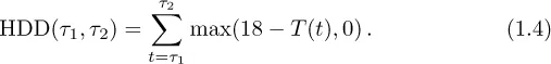
The HDD index, on the other hand, measures the demand for heating. It is mathematically defined as

One can imagine that households are putting on heating whenever the temperatures drop below 18°C. For example, a temperature of 0°C will give a HDD index of 18. The CDD and HDD indices are used for US and Australian cities as underlying for the temperature futures (using Fahrenheit as the unit of temperature). The futures are not settled on the index value for a particular day, but the aggregated index value over an agreed period of time, which we will refer to as the measurement period. The measurement periods are typically a week, month, or a longer period like two to seven consecutive months (then referred to as a seasonal strip). A seasonal strip is within the same general season, where winter is defined from October through April, and summer from April through October. For example, one could imagine a HDD index for New York measured over one week in January. If τ₁ is Monday of that week, and τ₂ is Sunday, then the HDD index for New York will be

If the observations for the week in question would be Monday 5°C, Tuesday 6°C, Wednesday 0°C, Thursday 10°C, Friday 12°C, Saturday 19°C and finally Sunday 19°C, the HDD index becomes

This would give a measurement of the demand of heating in New York for that given week. The HDD index is the underlying for futures contracts in the winter season.

A futures contract on a CDD or HDD index over a given measurement period is settled against the index value times a cash amount. For the US cities, this cash amount is USD20 per index point. In the above example, the buyer of the HDD futures will receive USD39 × 20, or USD780, in return for the agreed futures price....

Table of contents

• Front Cover
• Half Title
• Advances In Geosciences
• Title
• Copyright
• Editors
• Preface
• Contents
• 1. Financial markets for weather
• Statistics of weather
• 2. Data description and exploratory analysis
• 3. Spatial-temporal modelling
• Weather derivatives
• 4. Continuous-time models for temperature and wind speed
• 5. Pricing of forward contracts on temperature and wind speed
• 6. Extensions of temperature and wind speed models
• 7. Options on temperature and wind
• 8. Precipitation derivatives
• 9. Utility-based approaches to pricing weather derivatives
• Appendix
• Bibliography
• Index