Quantitative Modelling In Marketing And Management

Luiz Moutinho, Kun-Huang Huarng

• Publisher: WSPC
• Year: 2012
• Print ISBN: 9789814407717
• eBook ISBN: 9789814407731
• Topic: Biological Sciences
• Subtopic: Science General
• Index: Biological Sciences

The field of marketing and management has undergone immense changes over the past decade. These dynamic changes are driving an increasing need for data analysis using quantitative modelling.

Problem solving using the quantitative approach and other models has always been a hot topic in the fields of marketing and management. Quantitative modelling seems admirably suited to help managers in their strategic decision making on operations management issues. In social sciences, quantitative research refers to the systematic empirical investigation of social phenomena via statistical, mathematical or computational techniques.

This book focuses on the description and applications of many quantitative modelling approaches applied to marketing and management. The structure encompasses statistical, computer and mathematical as well as other models. The topics range from fuzzy logic and logical discriminant models to growth models and k-clique models. It also covers current research being conducted in the field.

Errata(s)
Errata (16 KB)

Contents:

• Statistical Modelling:
  • A Review of the Major Multidimensional Scaling Models for the Analysis of Preference/Dominance Data in Marketing (Wayne S DeSarbo and Sunghoon Kim)
  • Role of Structural Equation Modelling in Theory Testing and Development (Parikshat S Manhas, Ajay K Manrai, Lalita A Manrai and Ramjit)
  • Partial Least Squares Path Modelling in Marketing and Management Research: An Annotated Application (Joaquín Aldás-Manzano)
  • DEA — Data Envelopment Analysis: Models, Methods and Applications (Dr Alex Manzoni and Professor Sardar M N Islam)
  • Statistical Model Selection (Graeme D Hutcheson)
• Computer Modelling:
  • Artificial Neural Networks and Structural Equation Modelling: An Empirical Comparison to Evaluate Business Customer Loyalty (Arnaldo Coelho, Luiz Moutinho, Graeme D Hutcheson and Maria Manuela Santos Silva)
  • The Application of NN to Management Problems (Arnaldo Coelho, Luiz Moutinho and Maria Manuela Santos Silva)
  • Logical Discriminant Models (Margarida G M S Cardoso)
  • Meta-heuristics in Marketing (Stephen Hurley and Luiz Moutinho)
  • Hold a Mirror Up to Nature: A New Approach on Correlation Evaluation with Fuzzy Data and Its Applications in Econometrics (Chih Ching Yang, Yu-Ting Cheng, Berlin Wu and Songsak Sriboonchitta)
  • Non-parametric Test with Fuzzy Data and Its Applications in the Performance Evaluation of Customer Capital (Yu-Lan Lee, Ming-leih Wu and Chunti Su)
  • Too Much ADO About Nothing? Fuzzy Measurement of Job Stress for School Leaders (Berlin Wu and Mei Fen Liu)
  • Fuzzy Composite Score and Situational Judgement Test: An Integrated Operation Perspective of Scoring (Hawjeng Chiou and Tsung-Lin Ou)
• Mathematical and Other Models:
  • Cluster Analysis: An Example Analysis on Personality and Dysfunctional Customer Behaviour (Malcolm J Beynon and Kate L Daunt)
  • Assessing the Perception of Superstitious Numbers and Its Effect on Purchasing Intentions (Dina-Fu Chang and Yi-Sheng Jiang)
  • Qualitative Comparison Analysis: An Example Analysis of Clinical Directorates and Resource Management (Malcolm J Beynon, Aoife McDermott and Mary A Keating)
  • Data Mining Process Models: A Roadmap for Knowledge Discovery (Armando B Mendes, Luís Cavique and Jorge M A Santos)
  • Growth Models (Mladen Sokele)
  • PROMETHEE: Technical Details and Developments, and Its Role in Performance Management (Malcolm J Beynon and Harry Barton)
  • Clique Communities in Social Networks (Luís Cavique, Armando B Mendes and Jorge M A Santos)
  • Conclusion

Readership: Undergraduates and postgraduates of management and business administration, academic researchers marketing professionals, financial professionals and business consultants.

PART 1

STATISTICAL MODELLING

Chapter 1

A REVIEW OF THE MAJOR MULTIDIMENSIONAL SCALING MODELS FOR THE ANALYSIS OF PREFERENCE/DOMINANCE DATA IN MARKETING

Wayne S. DeSarbo^*
Smeal College of Business
Pennsylvania State University
University Park, PA.
[email protected]

Sunghoon Kim
Smeal College of Business
Pennsylvania State University
University Park, PA.
[email protected]

Multidimensional scaling (MDS) represents a family of various spatial geometric models for the multidimensional representation of the structure in data as well as the corresponding set of methods for fitting such spatial models. Its major uses in Marketing include positioning, market segmentation, new product design, consumer preference analysis, etc. We present several popular MDS models for the analysis of consumer preference or dominance data. The first spatial model presented is called the vector or scalar products model which represents brands by points and consumers by vectors in a T dimensional derived joint space. We describe both individual and segment level vector MDS models. The second spatial model is called the multidimensional simple unfolding or ideal point model where both brands and consumers are jointly represented by points in a T dimensional derived joint space. We briefly discuss two more complex variants of multidimensional unfolding called the weighted unfolding model and the general unfolding model. Here too, we describe both individual and segment level unfolding MDS models. We contrast the underlying utility assumptions implied by each of these models with illustrative figures of typical joint spaces derived from each approach. An actual commercial application of consideration to buy large Sports Utility Vehicle (SUV) vehicles is provided with the empirical results from each major type of model at the individual level is discussed.

Keywords: Multidimensional scaling; vector model; unfolding model; positioning analysis; market segmentation; clusterwise models.

1. Introduction

Using the Carroll and Arabie (1980) broad conceptualisation, we define multidimensional scaling (MDS) as a family of various geometric models for the multidimensional representation of the structure in data as well as the corresponding set of methods for fitting such spatial models. Carroll and Arabie (1980) present a taxonomy of the area of MDS based on the properties of the input measurement data (e.g., number of modes, number of ways, power of the mode, scale type, conditionality, completeness of the data, replications, etc.) and properties of the underlying multidimensional measurement model (e.g., type of geometric model, number of sets of points in the derived space, number of derived spaces, degree of constraints on model parameters, etc.). Thus, their definition extends classical MDS which typically deals only with spatial models for proximity data (e.g., similarities/dissimilarities) to various other forms of continuous and discrete representations, as well as to other data types. Our focus will be upon the two major types of models utilised for the analysis of dominance (i.e., preference, consideration to buy, choice, etc.) data as is typically collected in Marketing Research: The vector MDS model and the unfolding MDS model (Scott and DeSarbo, 2011). Readers interested in a more comprehensive discussion of this broad area of MDS are encouraged to consult the excellent book on MDS by Borg and Groenen (2005) for an in-depth treatment of these and other types of MDS approaches for the analysis of such data (e.g., correspondence analysis). For expositional purposes, we will assume that the data to be analysed is a two-way dataset of metric brand preferences where the rows of this data matrix (

) reflect a sample of consumers and the columns of the matrix represent brands in a designated product/service class. The general entry in this data matrix (P_ij) is the metric preference rating given for brand j by consumer i. The objective of the MDS models to be described is to estimate a spatial configuration (a joint space) of both row (consumers or derived market segments) and column (brands) objects such that their particular geometric interrelationships most parsimoniously recovers the input preference data

. We will describe both traditional individual level MDS models and more recent segment level or clusterwise MDS models for the analysis of such preference or dominance data.

2. The Vector MDS Model

2.1. The individual level vector MDS model

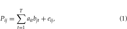
Tucker (1960) and Slater (1960) were the first to independently formulate this scalar products based model for geometrically displaying the structure in such two-way data (Carroll, 1972, 1980). Related to factor analysis, the underlying model can be mathematically represented as:

Where:

i = 1,…, I consumers;

j = 1,…, J brands;

t = 1,…, T dimensions;

a_it = the tth coordinate of the terminus of the preference vector for consumer i in the derived space;

b_jt = the tth coordinate of the location of brand j in the derived space;

_eij = error.

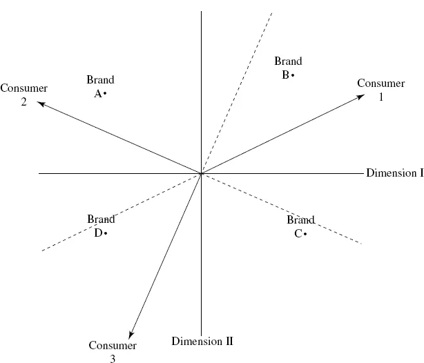
Fig. 1. The vector model.

We describe this particular geometric representation via, fig. 1 which illustrates the workings of the vector MDS model in Eq. (1) for the simple case of two dimensions, four brands, and three consumers. The two dimensions are labelled in the figure and represent typical scatter plot axes. The brand coordinates (b_jt) are plotted here for each of the four brands (A, B, C, and D) and represent the positions of the brands in this derived space. Note, the consumer locations (a_it) are represented in this model (labelled Consumers 1, 2, and 3) as vectors emanating thru the origin whose orientations point in the direction of increasing preference or utility for each consumer. Each of the three consumers’ vectors point in different directions reflecting heterogeneity (i.e., individual differences) in their respective tastes and preferences. (Note that we draw the tails of the vectors here as dashed lines reflecting the areas of the space that are dispreferred for each consumer). The predicted cardinal preference values are given by the orthogonal projection of each of the brands onto each consumer's preference vector. Thus, Consumer 1 has the following order of predicted preference: B, C, A, D; Consumer 2: A, D, B, C; and, Consumer 3: D, C, A, B. Note, the consumer vectors are typically normalised to equal length in such joint space representations although, under certain data preprocessing conditions, the raw lengths of such vectors can be shown to be proportional to how well each consumer's preferences are recovered by the vector representation. The goal of such an analysis is to simultaneously estimate the vectors and brand coordinates in a given dimensionality that most parsimoniously captures/recovers the empirical preference data. The analysis is typically repeated for t = 1,2,3,…, T dimensions and the dimensionality is selected by inspection of a scree plot of the number of estimated dimensions versus a goodness of fit statistic (e.g., variance accounted-for) that measures how well the model predictions in Eq. (1) match the input preference data given the number of model parameters being estimated. Note, the cosines of the angles each consumer vector forms with the coordinate axes render information relating to the importance of these derived dimensions to that consumer. The isopreference contours for this vector MDS model in two dimensions for a particular consumer vector (i.e., locations of equal preference) are perpendicular lines to a consumer vector at any point on that vector since brands located on such lines would project at the same point of predicted preference onto the vector. Thus, it is important to note that this vector model is not a distance based spatial model. Also, one can freely rotate the joint space of vectors and brand points and not change the model predictions (the orthogonal projections of the brand points onto the consumer vectors) or goodness-of-fit results. As noted by Carroll (1980), one of the unattractive features of this vector model is that it assumes that preference changes monotonically with respect to all dimensions. That is, since a consumer's vector points in the direction of increasing preference or utility, the more of the dimensions in that direction implies greater preference; i.e., the more the better. In marketing, this can create conceptual problems depending upon the nature of the underlying dimensions. This assumption may not be realistic for many latent attributes or dimensions underlying brands in a product/service class. For example, it is not clear that consumers prefer infinite amounts of size and sportiness (assuming those were the two underlying dimensions driving their vehicle preferences) in their family Sports Utility Vehicle (SUV). In addition, it would imply that the optimal positioning of new brands would be located towards infinity in the direction of these consumer vectors which is most often not realistic. However, the vector MDS model has been shown to be very robust and estimation procedures such as MDPREF (Carroll, 1972, 1980) based on singular value decomposition principles provide globally optimum results while being able to estimate all orthogonal dimensions in one pass of the analysis.

Recently, Scott and DeSarbo (2011) have extended this individual level deterministic vector MDS model to a parametric estimation framework and have provided four variants of the individual level vector MDS model involving reparameterisation options of the consumer and/or brand coordinates. There are occasions or application where the derived dimensional coordinates regarding

= ((a_it)) and/or

= ((b_jt)) in Eq. (1) are either difficult to interpret or need to be related to external information (e.g., brand attributes/features, subject demographics, etc.). One can always employ property fitting methods (Borg and Groenen, 2005) where methods such as correlation or multiple regression can be employed to relate

and/or

to such external information. Unfortunately, given the rotational indeterminacy inherent in the vector model, such methods can mask tacit relationships between these estimated dimensions and such external information. As such, the model defined in (1) can be generalised to incorporate additional data in the form of individual and/or brand background variables. The coordinates for individuals (vector termini) and/or brands, as the case might be, can be reparameterised as linear functions of background variables (see Bentler and Weeks, 1978; Bloxom, 1978; de Leeuw and Heiser, 1980; and Noma and Johnson, 1977, for constraining MDS spaces). If stimulus attribute data is available, then b_jt can be repara...

Table of contents

• Cover Page
• Title Page
• Copyright Page
• Contents
• Preface
• Introduction
• Part 1. Statistical Modelling
• Part 2. Computer Modelling
• Part 3. Mathematical and Other Models
• Index