![]()
PART 1
Mathematical Modeling in Epidemiology
![]()
Chapter 1
Epidemic Models
Epidemic models are usually used to study disease dynamics during a relatively short time period (e.g., within one year). In this case, the models often ignore processes that occur on longer time scales such as demographic processes (e.g., birth and death). Consequently, the models are usually simpler and easier for mathematical analyses. In this chapter, we focus primarily on the derivation of basic and control reproduction numbers and their relation to the final epidemic size. These quantities are important for designing control strategies. For discrete-time models, we also consider how model assumptions on the distribution of infectious stage may affect the estimates of reproduction numbers and final epidemic size. Particularly, we demonstrate that the commonly used simple discrete-time SIR or SEIR models implicitly assume that the infectious stage follows a geometric distribution, which is the only distribution with the memory-less property. When compared with models that assume more realistic sojourn distributions, the models provide contradictory predictions regarding the best control strategies. We provide an explanation for the apparent cause of the discrepant assessments.
This study reveals the importance of model assumptions. While memory-less distributions may be convenient mathematically, no biological process is memoryless. Evidently the information needed to characterize sojourn distributions must be collected (and if collected, reported) so that we can make realistic models. It would be hard to overestimate the importance of this. Models with arbitrarily distributed stage durations are also considered, from which formulas for the reproduction number and final epidemic size relation are derived. These formulas are expressed in terms of the probability quantities associated with the distribution, which makes the application of these models more easily particularly when disease data cannot be fitted well to any distributions from a particular parametric family.
1.1 Continuous-time models
Most continuous-time models are formulated using differential equations, including ordinary differential equations, partial differential equations, integral differential equations, among others. Several examples of such models are presented in this and later sections.
1.1.1 Simple SIR and SEIR epidemic models
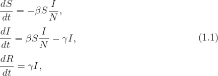
For the single-outbreak epidemic models presented in this section, some standard assumptions are adopted. The total population is divided into several epidemiological classes. For example, for an SIR model, the total population is divided into three epidemiological classes: susceptible (S), infectious (I), and recovered (R). Thus, in an ODE model (non-structured), the numbers of individuals in these classes at time t are S(t), I(t), and R(t), respectively, and the total number of individuals is N(t) = S(t)+I(t)+R(t). The force of infection (i.e., the number of new infections at time t) will take either the form of mass action, βSI, or the form of standard incidence, βSI/N, where β is a constant representing the infection rate per susceptible when contacting infectious individuals. This implies the assumption that the population mixing is homogeneous (i.e., no heterogeneities in age, gender, activity, susceptibility, infectiousness, etc.). If the infectious period is assumed to be exponentially distributed (see section 1.2.3 for models with more general distributions) with mean 1/γ, then γ gives the per-capita rate of recovery. It is also assumed that there are no disease deaths, so that the total population size remains constant for all time. Under these assumptions, the classical SIR epidemic model has the form
with initial conditions S(0) = S0, I(0) = I0 > 0, and R(0) = R0.This model is a special case of the general Kermack-McKendrick epidemic model (see [Brauer and Castillo-Chavez (2012)] for more details). The dynamical behavior of the model (1.1...