Uncertainty Within Economic Models

Lars Peter Hansen, Thomas J Sargent

• Publisher: WSPC
• Year: 2014
• eBook ISBN: 9789814578134
• Topic: Biological Sciences
• Subtopic: Science General
• Index: Biological Sciences

Written by Lars Peter Hansen (Nobel Laureate in Economics, 2013) and Thomas Sargent (Nobel Laureate in Economics, 2011), Uncertainty within Economic Models includes articles adapting and applying robust control theory to problems in economics and finance. This book extends rational expectations models by including agents who doubt their models and adopt precautionary decisions designed to protect themselves from adverse consequences of model misspecification. This behavior has consequences for what are ordinarily interpreted as market prices of risk, but big parts of which should actually be interpreted as market prices of model uncertainty. The chapters discuss ways of calibrating agents' fears of model misspecification in quantitative contexts.

Contents:

• Introduction
• Discounted Linear Exponential Quadratic Gaussian Control
• Robust Permanent Income and Pricing
• A Quartet of Semigroups for Model Specification, Robustness, Prices of Risk, and Model Detection
• Robust Control and Model Uncertainty
• Robust Control and Model Misspecification
• Doubts or Variability?
• Robust Estimation and Control without Commitment
• Fragile Beliefs and the Price of Uncertainty
• Beliefs, Doubts and Learning: Valuing Macroeconomic Risk
• Three Types of Ambiguity

Readership: Graduate students; researchers and economists interested in Econometrics; Macroeconomics and Dynamic Programming.
Key Features:

• A collection of papers adapting and applying robust control theory to problems in economics and finance
• Brings together works by two active researchers in the field and their coauthors
• Includes an introduction to link the papers and tell how they fit within broader efforts to improve macroeconomic and finance theories

Chapter 1

Introduction

1.1Questions about Model Uncertainty

These questions motivated us to write the chapters in this book.

What is model uncertainty?

For us, a model is a stochastic process, that is, a probability distribution over a sequence of random variables, perhaps indexed by a vector of parameters. For us, model uncertainty includes a suspicion that a model is incorrect.

Why do we care about it?

Because

•It is difficult statistically to distinguish alternative models from samples of the sizes of typical macroeconomic data sets.

•Experiments by Ellsberg (1961) make the no-model-doubts outcome implied by the Savage (1954) axioms dubious.

As macro econometricians, we will emphasize the first reason. Applied econometricians often emerge from model fitting efforts acknowledging substantial doubts about the validity of their models vis a vis nearly equally good fitting models. The second reason inspired decision theories that provides axiomatic foundations for some of the models applied in this book.¹

How do we represent it?

As a decision maker who has a set of models that he is unable or unwilling to reduce to a single model by using a Bayesian prior probability distribution over models to create a compound lottery.

How do we manage it?

We construct bounds on value functions over all members of the decision maker’s set of models. Min-max expected utility is our tool for constructing bounds on value functions. We formulate a two-player zero-sum game in which a minimizing player chooses a probability distribution from a set of models and thereby helps a maximizing player to compute bounds on value functions. This procedure explores the fragility of decision rules with respect to perturbations of a benchmark probability model.

Who confronts model uncertainty?

We as model builders do. So do the private agents and government decision makers inside our models.

How do we measure it?

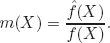
By the size of a set of statistical models, as measured by relative entropy. Relative entropy is an expected log likelihood ratio. For pedagogical simplicity, consider a static analysis under uncertainty. In fact it is the dynamic extensions that interest us, but the essential ingredients are present in this simpler setting. Let f(x) be a probability density for a random vector X under a benchmark model. Consider an alternative density

(x) for this random vector and form the likelihood ratio:

Provided that the support of the density

is contained in the support of the density f, the likelihood ratio m(X) has mean one under the benchmark f density:

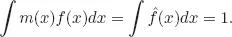
Posed differently, multiplication of f(x) by m(x) generates a perturbed probability density

(x) = m(x)f(x), since by construction

(x) integrates to 1. It is convenient for us to represent perturbed densities with positive functions m for which m(X) has expectation one. While we have assumed that the base-line probability distribution has a density with respect to Lebesgue measure, this is not needed for our analysis. We adopt the notational convention that expectations (not subject to qualification) are computed under the benchmark model f.

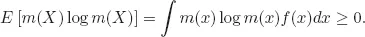
Relative entropy is defined as

Relative entropy equals zero when

(x) = f(x) and consequently m(x) = 1. Relative entropy tells how difficult it is to distinguish f(x) and

(x) with finite samples of x. It governs the rate of statistical learning as a sample size grows. Log likelihood ratios have been used to construct distinct but related quantities intended to measure discrepancies between probability distributions. We will discuss and occasionally use one of these due to Chernoff (1952). But relative entropy is the one that is most tractable for most of our analysis.

An urban legend claims that Shannon asked von Neumann what to call his mathematical object. Supposedly von Neumann said: “Call it entropy. It is already in use under that name and besides, it will give you a great edge in debates because nobody knows what entropy is anyway.” There are serious doubts about whether von Neumann actually said that to Shannon. The doubtful veracity of the story enhances its appropriateness for a book about model uncertainty.

How do we form a set of models?

In our simplest settings, we assume that a decision maker has a unique explicitly formulated statistical model f(x) that we often call an “approximating model” or “benchmark model.” We call it an approximating model to indicate that although it is the only explicitly formulated model possessed by the decision maker, he distrusts it. To express the decision maker’s doubts about his approximating model, we surround that model with all models that lie within an entropy ball of size η. The decision maker is concerned that some model within this set might actually govern the data.

We don’t specify particular alternative models with any detailed functional forms. We just characterize them vaguely with likelihood ratios whose relative entropies are less than η. In the applications to dynamic models described in this book, this vagueness leaves open complicated nonlinearities and history dependencies that are typically excluded in the decision maker’s approximating model. Nonlinearities, history dependencies, and false reductions in dimensions of parameter spaces are among the misspecifications that concern the decision maker.

Throughout much of our analysis, we use penalty parameters that scale relative entropy to capture the costs of evaluating outcomes using bigger sets of alternative models. The logic of the Lagrange multiplier theorem suggests a tight connection between so called “multiplier” formulations based on penalization and a related constraint formulation. The penalization formulation has some advantages from the standpoint of characterization and computation, but we often turn to an associated constraint formulation in order to assess quantitatively what degrees of penalization are plausible.

When we build models of learning in Chapters 8, 9, and 10, we explicitly put multiple benchmark models on the table. This gives the decision-maker something manageable to learn about. When learning is cast in terms of forming a weighted average over multiple models, an additional role for robustness emerges, namely, how to weight alternative models based on historical data in a way that allows for model misspecification.

How big is the set of models?

It is typically uncountable. In applications, an approximating model f(x) usually incorporates concrete low-dimensional functional forms. The perturbed models

(x) = m(x)f(x) do not. An immense set of likelihood ratios m(x), most of which can be described only by uncountable numbers of parameters, lie within an entropy ball E [m(X) log m(X)] ≤ η. The sheer size of the set of models and the huge dimensionality of individual models within the set make daunting the prospect of using available data to narrow the set of models.

Why not learn your way out of model uncertainty?

Our answer to this question comes from the vast extent and complexity of the set of models that a decision maker thinks might govern the data. All chapters in this book generate this set in the special way described above. First, we impute to the decision maker a single model that we refer to at different times either as his approximating model or his benchmark model. To capture the idea that the decision maker doubts that model, we surround it with a continuum of probability models that lie within a ball determined by entropy relative to the approximating model. That procedure gives the decision maker a vast set of models whose proximities to the approximating model are judged by their relative entropies.

We intentionally generate the decision maker’s set of models in this way because we want to express the idea that the decision maker is worried about models that are both vaguely specified and that are potentially difficult to distinguish from the approximating model with statistical discrimination tests. The models are vaguely specified in the sense that they are described only as the outcome of multiplying the approximating models probability density by a likelihood ratio whose relative entropy is sufficiently small. That puts on the table a huge number of models having potentially very high dimensional parameter spaces. These can include specifications that fluctuate over time, implying that relative to a benchmark model, later misspecifications differ from earlier ones. Learning which of these models actually governs the data generation is not possible without imposing more structure.²

As we shall see in applications in several chapters, specifications differentiated by their low frequency attributes are statistically especially difficult to distinguish (to learn those features, laws of large numbers and central limit theorems ask for almost infinite patience).³

More broadly, the fact that a decision maker entertains multiple possibly incorrect benchmark models puts us on unfamiliar ground in terms of an appropriate theory of learning. Bayesian learning theory assumes a decision maker who focuses on a set of models, one of which is correct. Bayes’ Theorem then tells how to update probabilities over models by combining prior information and data as intermediated through relative likelihoods.⁴ Positing that all candidate benchmark models are misspecified pushes us outside the Bayesian paradigm.

The applications in this book take two positions about learning. Chapters 2 through 7 exclude learning by appealing to the immense difficulty of learning. Chapters 8 and 9 describe and apply an approach to learning that imposes more structure on the decision maker’s model uncertainty.

How does model uncertainty affect equilibrium concepts?

To appreciate how model uncertainty affects standard equilibrium concepts, first think about the now dominant rational expectations equilibrium concept. A rational expectations model is shared by every agent inside the model, by nature, and by the econometrician (please remember that by a model, we mean a probability distribution over a sequen...

Table of contents

• Cover Page
• Title Page
• Copyright Page
• Dedication Page
• Contents
• Foreword
• Preface
• Acknowledgements
• About the Authors
• List of Figures
• List of Tables
• 1. Introduction
• 2. Discounted Linear Exponential Quadratic Gaussian Control
• 3. Robust Permanent Income and Pricing
• 4. A Quartet of Semigroups for Model Specification, Robustness, Prices of Risk, and Model Detection
• 5. Robust Control and Model Uncertainty
• 6. Robust Control and Model Misspecification
• 7. Doubts or Variability?
• 8. Robust Estimation and Control without Commitment
• 9. Fragile Beliefs and the Price of Uncertainty
• 10. Beliefs, Doubts and Learning: Valuing Macroeconomic Risk
• 11. Three Types of Ambiguity
• Bibliography
• Author Index
• Subject Index