Dark Energy

Miao Li, Xiao-Dong Li, Shuang Wang, Yi Wang

• Publisher: WSPC
• Year: 2014
• eBook ISBN: 9789814619721
• Topic: Biological Sciences
• Subtopic: Science General
• Index: Biological Sciences

This book introduces the current state of research on dark energy. It consists of three parts. The first part is for preliminary knowledge, including general relativity, modern cosmology, etc. The second part reviews major theoretical ideas and models of dark energy. The third part reviews some observational and numerical works. The aim of this book is to provide a sufficient level of understanding of dark energy problems, so that the reader can both get familiar with this area quickly and also be prepared to tackle the scientific literature on this subject. It will be useful for graduate students and researchers who are interested in dark energy.

Contents:

• Preliminaries in a Nutshell:
  • Gravitation
  • Matter Components
  • Cosmology
• Theoretical Aspects:
  • Introduction to Dark Energy
  • Weinberg's Classification
  • Symmetry
  • Anthropic Principle
  • Tuning Mechanisms
  • Modified Gravity
  • Quantum Cosmology
  • Holographic Principle
  • Back-Reaction
  • Phenomenological Models
  • The Theoretical Challenge Revisited
• Observational Aspects:
  • Basis of Statistics
  • Cosmic Probes of Dark Energy
  • Dark Energy Projects
  • Observational Constraints on Specific Theoretical Models
  • Dark Energy Reconstructions from Observational Data

Readership: Graduate students and researchers interested in Astrophysics and Cosmology.
Key Features:

• This book presents comprehensive overview of theoretical and observational aspects of research on dark energy.
• Almost all of major works on this area are introduced.
• Students and Researchers can use this like a handbook

Part I

Preliminaries in a Nutshell

1

Gravitation

For a quick review of gravitation, we start from the equations of Newtonian gravity. The gravitational force acting on a test mass m is

where Φ is called the Newtonian potential, which is determined by the Poisson equation

where ρ describes the mass distribution of a gravitational source, and G is the Newton’s gravitational constant.

Newtonian gravity captures some features of our universe. However, mass sums up. As a result, on cosmological scales, Newtonian gravity breaks down. For a systematic description of our universe, the theory of general relativity is inevitably required.

In the remainder of this chapter we briefly review the two key concepts in general relativity: what if spacetime is curved and what makes spacetime curved. Here we are by no means trying to provide a logical introduction for general relativity. Instead, we pragmatically highlight parts of the theory which are building blocks for a phenomenological description of dark energy, as well as set up our conventions.

1.1The Curved Spacetime

It is for a long time a great mystery why our space is well described by Euclidean geometry. In the spatial two dimensional story, numerous attempts are made to prove the “parallel axiom” and eventually the axiom turns out not provable. Instead, Euclidean geometry only applies for flat slicings, and the parallel axiom is the additional assumption to be made.

In the 3-dimensional space story, similarly the fact that our spatial dimensions are well described by Euclidean geometry is not for granted but instead has profound implications in physics, which in part leads to the discovery of cosmic inflation. Moreover, in the 3 + 1 dimensional story, when time is also considered, the geometry of spacetime is proven not flat on cosmological spacetime scales. Thus a description of curved spacetime is an essential in modern cosmology.

For two dimensional curved space, an intuitive understanding can be obtained by embedding into 3 dimensions. However, to investigate our curved spacetime, it is more convenient to use an intrinsic description instead of the embedding way. This is because on the one hand, we do not have good intuition on higher dimensions where our spacetime can be embedded into, and on the other hand, although such embeddings always exist in mathematics, there is no evidence for their physical existence.

The metric is what one needs to construct an intrinsic description of spacetime. A proper length between two nearby points can be defined as

where g_μν(x) is the metric, which describes the geometry of spacetime. We require the metric to be symmetric: g_μν = g_νμ, because the anti-symmetric part does not contribute as long as dx^μ and dx^ν commute.

Our spacetime is Lorentzian. In other words, there is one time dimension and all the other dimensions are spatial. The metric takes different sign between the two. The sign convention we use here is (−, +, +, +). Greek labels as μ and ν take value in these dimensions, and repeated labels are by default summed (Einstein’s convention).

The affine connection (also known as the Christoffel symbol), describing how a vector moves along a curve, is defined as

where ∂_μ is a shorthand for partial derivative ∂/∂x_μ. The affine connection is symmetric about the two lower indices: Γ^λ_μν = Γ^λ_μν.

Covariant derivatives can be constructed using the connection as

where ϕ is a scalar field, and A_ν and A^ν are vector fields with lower and upper indices respectively. Covariant derivatives of higher rank tensors can be constructed similarly.

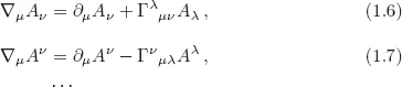
The Riemann curvature tensors can be constructed based on the metric, the affine connection and their derivatives. Among those the most useful ones are the Riemann tensor R^ρ_σμν, the Ricci tensor R_μν, and the Ricci scalar

, defined as

Note that R_μν = R_νμ is symmetric.

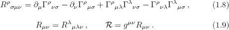
A free particle (which is not affected by any other force except gravitation) moves following a line that extremizes its proper distance. Such a line is called a geodesic. Supposing the free particle moves along a world line x^μ(λ), the world line satisfies the geodesic equation

Defining four velocity u^ρ ≡ dx^ρ/dλ, the geodesic equation can also be written as

It is in principle arbitrary to choose the parameterization λ. However for massive particles a particular convenient choice is dλ = dτ, where τ is the proper time. This choice of λ is called affine parameter and in this case the four velocity is normalized to u^μu_μ = −1.

1.2The Curved Spacetime: An Example

Here we illustrate the concepts of the last section by considering an explicit (and useful) example. Consider the metric called “spatially flat Friedmann–Robertson–Walker metric”:

where c is the speed of light. Hereafter, unless otherwise noted, we will take c = 1. The nonzero components of the connection can be worked out as

where

is the Hubble parameter. The dot on a variable denotes time derivative. The value of H at the present epoch (denoted as H₀) is called the Hubble constant.

The components of the Ricci tensor are

and the Ricci scalar takes the form

The kinematics of a massless particle can be derived from the geodesic equation. Or alternatively, here we use a simpler method: a m...

Table of contents

• Cover page
• Title Page
• Copyright
• Foreword
• Preface
• Contents
• Part I Preliminaries in a Nutshell
• Part II Theoretical Aspects
• Part III Observational Aspects
• Index