![]()
Chapter 1
Introduction
A particle of mass m which is displaced from its equilibrium position at x = 0 is subject to a restoring attractive force and a viscous force which, in first approximation, are proportional to the displacement and velocity, respectively. Thus, for an one-dimensional system, Newton’s law gives
where 2γ/m is the damping rate and ω/m1/2 is the intrinsic frequency. The solution of this equation is
where
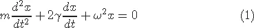
If the harmonic oscillator is subject to an external periodic force A exp(iΩt),
then the complete solution of this equation consists of solution (2) of the homogeneous equation (1) and the following solution of the non-homogeneous equation,
The last equation indicates the possibility of a (dynamic) resonance, when the external frequency Ω approaches the intrinsic frequency ω/m1/2.
1.1Harmonic oscillator with external noise
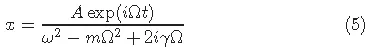
In the foregoing we considered a pure mechanical system (zero temperature). For non-zero temperatures, the dynamic equation (1) has to be supplemented by the thermal noise
where η(t) is the random variable with zero mean, 〈η(t)〉 = 0, and variance 〈η2(t)〉, which for thermal noise satisfies the fluctuation-dissipation theorem 〈η2(t)〉 = 4γκT, where κ is the Boltzmann constant [2]. The latter simply means that the power entering the system from the external force must be entirely dissipated and given off to the thermostat in order that the equilibrium state of the system not be disturbed. Another way to justify the validity of Eq. (6) is as follows: in considering only one (slow) mode x(t) of a complex system, one may take into account the influence of other (fast) modes by introducing a random force into dynamic equation with no special requirements for the value of 〈η2(t)〉.
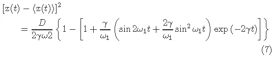
Upon averaging Eq. (6), one finds that the first moment is given by Eq. (2) while the second moment 〈x2(t)〉 for white noise 〈η2(t)〉 = D is defined by the variance,
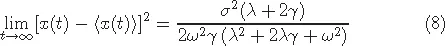
For m = 1, dichotomous noise of strength σ2 and inverse correlation length λ, the variance reaches the following stationary (t → ∞) value
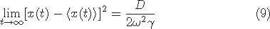
which for white noise is reduced to
Both equations (7) and (8) were obtained already in 1945 [3].
1.2Ito-Stratonovich dilemma
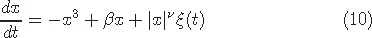
In spite of the fact that the stochastic differential equations were introduced more than a hundred years ago, there are still many interesting problems concerning these equations. We consider here the Ito-Stratonovich dilemma, using the generalized Schlogl model as an example [4], which is described by the following equation,
where ν is an arbitrary number and ξ(t) is white noise with the correlator
The Langevin equation (10) is not completely defined due to the Ito–Stratonovich dilemma, namely, it is not clear which value of t one has to insert in the δ-function (11) and afterwards in the probability distribution. The two possibilities are: before the jump (Ito) or the averaged of before and after the jump (Stratonovich). This choice is very important since it leads to different Fokker-Planck equation for the probability distribution P(x, t) [5]. The first is described by the dynamic equation of the form
and the second by the equation
Another important factor which defines the behavior of a system is the value of ν.
1.
For
ν = 0, there are three steady states for
β > 0, namely,
x0 = 0 (unstable) and
(stable), and one stable state for
β < 0, namely,
x0 = 0.
2.For ν > 0, multiplicative noise has an attractive effect, i.e., it attracts the probability P(r, t) to unstable steady state, whereas for ν < 0, the noise term makes system more stable.
3.The stationary probability distribution P(x) (at t → ∞) is defined by the competition between the noise and the damping terms in Eq. (10), which define in going and outgoing energy, respectively, i.e., by three numbers, ν, β and D. In the Stratonovich approach [4] P (x) = C exp ...