![]()
Chapter 1
A Few Introductory Problems
Even if deterministic Calculus is an excellent tool for modeling real life problems, however, when it comes to random exterior influences, Stochastic Calculus is the one which can allow for a more accurate modeling of the problem. In real life applications, involving trajectories, measurements, noisy signals, etc., the effects of many unpredictable factors can be averaged out, via the Central Limit Theorem, as a normal random variable. This is related to the Brownian motion, which was introduced to model the irregular movements of pollen grains in a liquid.
In the following we shall discuss a few problems involving random perturbations, which serve as motivation for the study of the Stochastic Calculus introduced in next chapters. We shall come back to some of these problems and solve them partially or completely in Chapter 11.
1.1Stochastic Population Growth Models
Exponential growth model Let P(t) denote the population at time t. In the time interval Δt the population increases by the amount ΔP(t) = P(t + Δt) − P(t). The classical model of population growth suggests that the relative percentage increase in population is proportional with the time interval, i.e.
where the constant r > 0 denotes the population growth. Allowing for infinitesimal time intervals, the aforementioned equation writes as
This differential equation has the solution P(t) = P0ert, where P0 is the initial population size. The evolution of the population is driven by its growth rate r. In real life this rate is not constant. It might be a function of time t, or even more general, it might oscillate irregularly around some deterministic average function a(t):
In this case, rt becomes a random variable indexed over time t. The associated equation becomes a stochastic differential equation
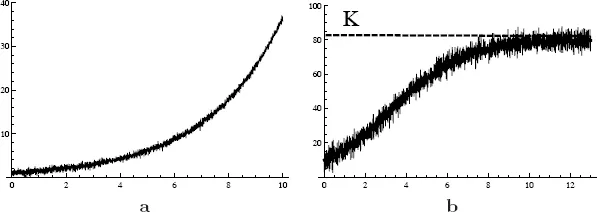
Solving an equation of type (1.1.1) is a problem of Stochastic Calculus, see Fig. 1.1(a).
Figure 1.1: (a) Noisy population with exponential growth. (b) Noisy population with logistic growth.
Logistic growth model The previous exponential growth model allows the population to increase indefinitely. However, due to competition, limited space and resources, the population will increase slower and slower. This model was introduced by P.F. Verhust in 1832 and rediscovered by R. Pearl in the twentieth century. The main assumption of the model is that the amount of competition is proportional with the number of encounters between the population members, which is proportional with the square of the population size
The solution is given by the logistic function
where K = r/k is the saturation level of the population. One of the stochastic variants of equation (1.1.2) is given by
where
is a measure of the size of the noise in the system. This equation is used to model the growth of a population in a stochastic, crowded environment, see
Fig. 1.1(b).
1.2Pricing Zero-coupon Bonds
A bond is a financial instrument which pays back at the end of its lifetime, T, an amount equal to B, and provides some periodical payments, called coupons. If the co...