Physics Matters

Vasant Natarajan

• Publisher: WSPC
• Year: 2016
• eBook ISBN:
  9789813142534
• Topic: Physical Sciences
• Subtopic: Optics & Light

This is a collection of essays on physics topics. It is written as a textbook for non-physics science and arts students, at the undergraduate level. Topics covered include cellphone radiation, lasers, the twin paradox, and more.

Contents:

• Oscillations
• The Myth of Cell Phone Radiation
• What Einstein Meant When He Said "God Does Not Play Dice..."
• Einstein as Armchair Detective — The Case of Stimulated Radiation
• Standards for Units
• The Twin Paradox in Relativity
• Robert Dicke and Atomic Physics
• The 1997 Nobel Prize in Physics — Laser Cooling and Trapping
• The 2001 Nobel Prize in Physics — Bose–Einstein Condensation
• The 2005 Nobel Prize in Physics — Laser Physics
• The 2009 Nobel Prize in Physics — Achievements in Optics That Have Changed Modern Life
• The 2012 Nobel Prize in Physics — Manipulation of Single Particles

Readership: Non-physics undergraduates in both the sciences and the arts.

Chapter 1

Oscillations

ALMOST all undergraduate textbooks on physics treat the simple harmonic oscillator in detail because it is the key to understanding much of physics. Apart from direct applications such as in a pendulum clock, it can be used to understand collective excitations like phonons in a solid. But perhaps the most important reason to study them is that it is first step in understanding light. A light wave is like a harmonic oscillator, except that instead of position and velocity oscillating as in a mechanical oscillator, it is the electric and magnetic fields that oscillate in a light wave.In addition, as we will see in this chapter, it can be used to understand many phenomena that are normally associated with quantum mechanics. The reason for this is that the main equation governing quantum mechanics is the Schrödinger equation, which is just a modified wave/oscillator equation.

A. The simple pendulum

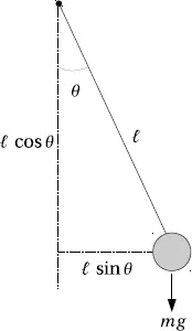
We first analyze the dynamics of the simple pendulum, mainly because it is slightly different from the normal application of Newton’s second law of motion F = ma. As shown in Fig. 1.1, the dynamical variable in the pendulum is the angle θ and not the position x. This implies that the acceleration has dimensions of [T]⁻², which means that the dimensions of the inertial term has to be [M][L]² in order to get the dimensions of force correct. The modified equation of motion is therefore

where τ is the torque (moment of force) about the point of contact, and I = mℓ² is the moment of inertia of the pendulum bob about the point of contact. The torque is given by

The minus sign is because the torque is in the −θ direction.

Figure 1.1: Simple pendulum showing relevant parameters used in the analysis.

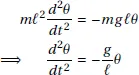
Using the small angle approximation that sin θ ≈ θ in the equation of motion, we get

This is the familiar harmonic oscillator equation of motion. Its general solution—which can be verified by substitution—is given by

Here θ₀ is the amplitude of the motion, φ is the phase at t = 0, and

is the (angular) frequency of the oscillator. θ₀ and φ are determined by the initial conditions, i.e. initial position and initial velocity of the bob—two constants in the solution because the equation of motion is a second order equation.

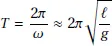
The defining characteristic of harmonic motion is that the frequency is independent of amplitude. In the case of the simple pendulum, this is true only when the angle is small, so that sin θ can be approximated as θ. The time period of motion T (defined as the time taken for one complete cycle) is written as

independent of amplitude θ₀. For larger amplitudes, T becomes a function of θ₀, and the oscillator is called “anharmonic”. A Taylor expansion of the sin term in the equation of motion then yields

which shows explicitly that the time period increases at larger amplitudes.

This behavior can be understood from the shape of the potential energy curve. For a conservative force like that due to gravity, the force can be derived from a potential U as follows

Geometric analysis of the force on the pendulum bob shown in Fig. 1.1 gives for the potential

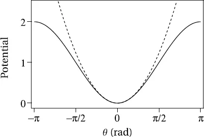
This potential (with mgℓ = 1) is shown in Fig. 1.2 for a range of −π to +π. A Taylor expansion of the potential around θ = 0 yields

The first term in this expansion is the parabolic or harmonic term, for which the small angle approximation is valid. For comparison, this parabolic shape is also shown in the figure (as a dotted line). It is seen that the real potential is shallower than the harmonic one.

The motion in the full potential will remain periodic, i.e. return to the same point in the potential curve, because the system has no way of losing energy. However, it will not be sinusoidal—have a single frequency component—as in the case of a harmonic oscillator. Furthermore, in accordance with Eq. (1.3), the time period will increase with amplitude.

Figure 1.2: Shape of the potential seen by the pendulum bob. For comparison, the parabolic approximation near θ = 0 is shown with a dotted line.

B. Parametric amplification

Parametric amplification is a method to amplify the motion by modulating some parameter of the system at twice the natural frequency. This is different from normal amplification, where the amplitude is increased by a periodic driving force at the oscillation frequency.

The idea behind parametric amplification can be understood by considering the motion of a child on a swing. After playing on it for a while, she learns to increase her amplitude by instinctively crouching at the bottom—thereby increasing the length of the swing—and stretching at the ends—thereby decreasing the length of the swing—thus changing the length twice every period. This is a method of self-amplification which does not require contact with ground or boosts from another person. The parameter of the swing (or the equivalent pendulum) that is being changed at is the length, which from Eq. (1.2) determines ω.

Mathematically, the potential becomes

the first term is the normal harmonic oscillator potential that we saw earlier. The second term arises because the length is modulated at twice the natural frequency—i.e. frequency modulation at 2ω. The degree of modulation, determined by ε, is considered small—i.e. ε

1. The corresponding equation of motion is

since ε is small, we get the solution

this is the standard solution for the motion of a pendulum, as can be verified by expanding the solution in Eq. (1.1), except that B and C are not constants but functions of time. But their time variation is taken to be slow enough that the second derivative can be neglected. Therefore

Substituting into the equation of motion in Eq. (1.4), we get

Using trigonometric identities and averaging away the terms rapidly oscillating at 3ω, yields

The coefficients of the sin and cos terms must be separately equal, which gives

Solving the above yields

This shows that the amplitude of the cos quadrature increases exponentially with time, while the sin quadrature decreases by the same factor. The amplitude of the motion

increases with time—the signature of any amplification process.

1. Squeezed states

The above discussion of parametric amplification leads us to another concept in quantum mechanical states of light, namely squeezed states. The light wave, like a harmonic oscillator, has two degrees of freedom—the sin and cos components of the electric (or magnetic) field. Each of these has a mean squared value determined by the Heisenberg uncertainty principle, which are equal for the ground or vacuum state. The uncertainty distribution in phase space—with sin and cos axes—is circularly symmetric. This can be “squeezed” along some axis, so that the distrib...

Table of contents

• Cover page
• Title page
• Copyright
• Dedication
• Contents
• Abbreviations
• Preface
• Acknowledgments
• About the Author
• 1. Oscillations
• 2. The myth of cell phone radiation
• 3. What Einstein meant when he said “God does not play dice ...”
• 4. Einstein as armchair detective—The case of stimulated radiation
• 5. Standards for units
• 6. The twin paradox in relativity
• 7. Robert Dicke and atomic physics
• 8. The 1997 Nobel Prize in Physics—Laser Cooling and Trapping
• 9. The 2001 Nobel Prize in Physics—Bose-Einstein condensation
• 10. The 2005 Nobel Prize in Physics—Laser physics
• 11. The 2009 Nobel Prize in Physics—Achievements in optics that have changed modern life
• 12. The 2012 Nobel Prize in Physics—Manipulation of single particles
• Index