Great Investment Ideas

William T Ziemba

• Publisher: WSPC
• Year: 2016
• Topic: Business
• eBook ISBN:
  9789813144392
• Subtopic: Financial Engineering
• Index: Business

-->

Great Investment Ideas is a collection of articles published in the Journal of Portfolio Management from 1993 to 2015. The book contains useful ideas for investment management and trading and discusses the methods, r

Chapter 1

Comment on “Why a Weekend Effect?”^∗

William T. Ziemba

University of British Columbia,
Vancouver, BC V6T 1Y8, Canada
and
The Yamaichi Research Institute, Tokyo, Japan

The weekend effect in U.S. security markets has been documented by French (1980), Gibbons and Hess (1981), and others. Miller (1988) argues that the effect could be explained by a tendency for self-initiated sell orders to exceed self-initiated buy orders over the weekend, while broker-initiated buy trades result in a surplus of buying during the remainder of the week.

This causes security prices to fall over the weekend and during the day on Monday as market makers sell back stock on the open. Prices then move higher during the week because of broker-induced buying. Osborne (1962) presents a similar hypothesis, which also argues that institutional investors are less active on Mondays as effort is made that day to plan the week’s trades.

The day-of-the-week variation is higher for small-capitalized than for large-capitalized firms because of the larger bid-ask spreads and the thin trading in these generally low-priced securities. Keim and Smirlock (1987) document this for U.S. markets, and Stoll and Whaley (1983) confirm the bid-ask spreads.

Miller’s idea is predicated on the fact that people are simply too busy to think much about stocks during the week. If they do anything, it’s more often than not to buy upon the recommendation of a broker. Brokers have a vested interest in purchases. First, they do not have to find people who own stock and suggest they sell it. Second, they reveive two commissions for the purchases (usually recommended by the broker) and the sale (usually initiated by the stock owner).

Groth et al. (1979) survey 6,000 broker recommendations. Eighty-seven percent represent purchase and only 13% sales recommendations. Dimson and Marsh (1986) report similar recommendations by U.K. financial analysts. As individual investors think about their holdings over the weekend, they tend more to sell than to buy. Individuals, on balance, are net sellers of stock.

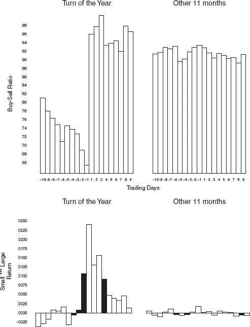
Exhibit 1 from Ritter (1988) illustrates buy-sell ratios with data on individual orders at Merrill Lynch for January and the rest of the year between 1971 and 1985. There is also a strong turn-of-the-year effect for small stocks on trading days −1 to +4.

Although Miller’s story is plausible, he did not test the theory with real data. Lakonishok and Maberly (1990) have provided such a test with New York Stock Exchange (NYSE) odd-lot sales and purchases, sales and purchases of cash-account customers of Merrill Lynch, and NYSE block transactions. They find that Monday has the lowest trading volume. Insititutional trading is the lowest on Monday of all trading days, but individual trading on Monday is the highest relative to other days of the week.

Individuals also sell more on Mondays. For example, odd-lot sales minus odd-lot purchases relative to NYSE volume were 29% higher during 1962–1986 on Monday than for the average of Tuesday to Friday.

Theoretical support for imbalances on different days in trading volume, mean returns, and volatility based on the interaction of various traders has been advanced by Admati and Pfleiderer (1988, 1989).

Day-of-the-Week Effects

Previous, studies of holiday effects in Japanese spot and futures markets reveal strong and significant positive preholiday effects and negative post-holiday effects over the 1949–1988 period (Ziemba 1989; 1991). Hence it is appropriate to separate out the day-of-the-week effects.

Additional research on day-of-the-week effects in Japan appears in Jaffe and Westerfield (1985), Kato (1990), Kato, Schwartz, and Ziemba (1990), and Ziemba and Schwartz (1991). Recent research on Japanese financial markets is surveyed in Ziemba, Bailey, and Hamao (1991).

EXHIBIT 1: Mean Buy/Sell Ratios and the Excess Return on Small Stocks by Trading Day in January and the Rest of the Year, 1971–1985.

Source: Ritter (1988).

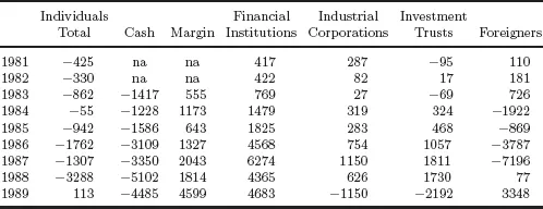
EXHIBIT 2: Net Purchases (Sales) of Stocks in Billions of Yen February by Various Investor Groups, 1981–1989.

Source: Yamaichi Research Institute.

This article investigates the weekend hypothesis for the Japanese market using daily data from May 16, 1949, to December 28, 1988. The data are broken into 475 ten-year subperiods beginning with May 1949 to April 1958 and ending with January 1979 to December 1988. Exhibit 2 shows that individual investors were net sellers in Japan as well as the U.S. during 1981–1989.

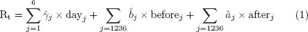
For each of the 475 ten-year periods the equation is estimated.

The coefficients aj refer to the single trading days that are after aj = 1, j = 2, j = 3, and j = 6-day break from a trading holiday or weekend. Similarly, the bjs refer to the single trading day before a 1, 2, 3, or 6-day break from trading. Hence Equation (1) gives as coefficients γ_j for the six days of the week the pure effects of these days separate from the holiday and weekend effects.

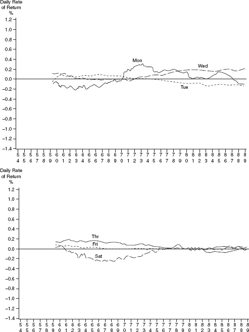
Exhibit 3 gives the mean returns by day of the week estimated from Equation (1) after adjusting for pre- and post-holiday effects by year from 1949 to 1988. Each ten-year period is plotted at its final month. For example, May 1949 to April 1958 is ploted as April 1958.

Hence there are 475 such points for Monday, Tuesday, to Saturday in the estimate of γ₁ to γ₆ in Equation (1) for that ten-year period. The 475 points represent partially overlapping periods over the more than thirty-nine years of data.

EXHIBIT 3: Day-of-the-Week Effects by Ten-year Period Ending in the Plotted Month for Periods Ending in April 1958 to December 1988 with Holiday and Weekend Effects Separated Out.

Source: Yamaichi Research Institute.

Exhibit 4 shows the test of hypotheses by day of the week that the daily return is not zero for each of the months in the years of the sample May 1949 to December 1988. Most of the time the daily return is not zero (i.e., it is above the line) at the 5% significance level.

Testing Miller’s Hypothesis

A test of a hypothesis along the lines of Miller’s is shown in Exhibit 5 with P-statistics in Exhibit 6. Here P refers to the probability of accepting a false hypothesis using a two-tail test. Miller’s argument implies that individual investors reach net sell decisions on each weekend day (when they are not being urged to buy by brokers). These net decisions to sell made on the weekend come to market on Mondays, tending to force the price down.

This theory implies that Monday declines after two days free of broker calls should be greater than after one day. The Japanese data provide a chance to test this prediction because some weekends provide only one day free of broker’s calls, and other weekends two such days.

Case A₁ refers to the one-day weekends following weeks with Saturday trading, and A₂ refers to the two-day weekends. The coefficients â₁ and â₂ are from Equation (1) for each of the 475 ten-year overlapping periods. The hypothesis is that the average returns on the A₂ days are lower than those on the A₁ days.

Exhibit 5 confirms this, showing Monday’s average daily returns for the 475 ten-year periods. P-values for the hypothesis that the return on Monday is not zero using a two-tailed test appear in Exhibit 6.

One-Versus Two-Day Weekends

Sales efforts are intensified before holidays and weekends, which results in high returns on the preholiday Fridays and Saturdays. Exhibit 7 shows that the daily rise before two-day holidays and weekends is larger than far one-day breaks from trading using the

and

coefficients. Exhibit 8 gives the P-values for the sample period 1954–1989.

The results provide further evidence that Monday returns (based on the time between the close of the previous week’s trading and the end of Monday’s) do not relate to a time in the investment cycle that would predict high re...

Table of contents

• Cover Page
• World Scientific Series in Finance
• Title
• Copyright
• Contents
• Preface
• Acknowledgements
• 1. Comment on “Why a Weekend Effect?”
• 2. The Effect of Errors in Means, Variances, and Covariances on Optimal Portfolio Choice
• 3. The Turn-of-the-Month Effect in the U.S. Stock Index Futures Markets, 1982–1992
• 4. Stock Ownership Decisions in Defined Contribution Pension Plans
• 5. The Symmetric Downside-Risk Sharpe Ratio and the Evaluation of Great Investors and Speculators
• 6. The Predictive Ability of the Bond Stock Earnings Yield Differential Model
• 7. Do Seasonal Anomalies Still Work?
• 8. How Does the Fortune’s Formula-Kelly Capital Growth Model Perform?
• 9. Great Investors: Their Methods, Results and Evaluation
• 10. Is the 60-40 Stock-Bond Pension Fund Rule Wise?
• 11. When to Sell Apple and the NASDAQ? Trading Bubbles with a Stochastic Disorder Model
• 12. A Response to Professor Paul A. Samuelson’s Objections to Kelly Capital Growth Investing
• Index