Differential Equations as Models in Science and Engineering

Gregory Baker

• Publisher: WSPC
• Year: 2016
• ISBN:
  9789814656993
• Topic: Matemáticas
• Subtopic: Ecuaciones diferenciales

This textbook develops a coherent view of differential equations by progressing through a series of typical examples in science and engineering that arise as mathematical models. All steps of the modeling process are covered: formulation of a mathematical model; the development and use of mathematical concepts that lead to constructive solutions; validation of the solutions; and consideration of the consequences. The volume engages students in thinking mathematically, while emphasizing the power and relevance of mathematics in science and engineering. There are just a few guidelines that bring coherence to the construction of solutions as the book progresses through ordinary to partial differential equations using examples from mixing, electric circuits, chemical reactions and transport processes, among others. The development of differential equations as mathematical models and the construction of their solution is placed center stage in this volume.

Linear Ordinary Differential Equations

1

1.1Growth and decay

A good starting point is to see just how differential equations arise in science and engineering. An important way they arise is from our interest in trying to understand how quantities change in time. Our whole experience of the world rests on the continual changing patterns around us, and the changes can occur on vastly different scales of time. The changes in the universe take light years to be noticed, our heart beats on the scale of a second, and transportation is more like miles per hour. As scientists and engineers we are interested in how specific physical quantities change in time. Our hope is that there are repeatable patterns that suggest a deterministic process controls the situation, and if we can understand these processes we expect to be able to affect desirable changes or design products for our use.

We are faced, then, with the challenge of developing a model for the phenomenon we are interested in and we quickly realize that we must introduce simplifications; otherwise the model will be hopelessly complicated and we will make no progress in understanding it. For example, if we wish to understand the trajectory of a particle, we must first decide that its location is a single precise number, even though the particle clearly has size. We cannot waste effort in deciding where in the particle its location is measured,¹ especially if the size of the particle is not important in how it moves. Next, we assume that the particle moves continuously in time; it does not mysteriously jump from one place to another in an instant. Of course, our sense of continuity depends on the scale of time in which appreciable changes occur. There is always some uncertainty or lack of precision when we take a measurement in time. Nevertheless, we employ the concepts of a function changing continuously in time (in the mathematical sense) as a useful approximation and we seek to understand the mechanism that governs its change.

In some cases, observations might suggest an underlying process that connects rate of change to the current state of affairs. The example used in this chapter is bacterial growth. In other cases, it is the underlying principle of conservation that determines how the rate of change of a quantity in a volume depends on how much enters or leaves the volume. Both examples, although simple, are quite generic in nature. They also illustrate the fundamental nature of growth and decay.

1.1.1Bacterial growth

The simplest differential equation arises in models for growth and decay. As an example, consider some data recording the change in the population of bacteria grown under different temperatures. The data is recorded as a table of entries, one column for each temperature. Each row corresponds to the time of the measurement. The clock is set to zero when the bacteria is first placed into a source of food in a container and measurements are made every hour afterwards. The experimentalist has noted the physical dimensions of the food source. It occupies a cylindrical disk of radius 5 cm and depth of 1 cm. The volume is therefore 78.54 cm³. The population is measured in millions per cubic centimeter, and the results are displayed in Table 1.1.

Table 1.1 Population densities in millions per cubic centimeters.

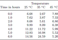
Glancing at the table, it is clear that the populations increase in the first two columns but decay in the last. Detailed comparison is difficult because they do not all start at the same density. That difficulty can be easily remedied by looking at the relative densities. Divide all the entries in each column by the initial density in the column. The results are displayed in Table 1.2 as the change in relative densities, a quantity without dimensions. Since we use the ...