Problems in Portfolio Theory and the Fundamentals of Financial Decision Making

Leonard C MacLean, William T Ziemba

• Publisher: WSPC
• Year: 2016
• eBook ISBN:
  9789814759366
• Topic: Betriebswirtschaft
• Subtopic: Finanzwesen

-->

This book consists of invaluable introductions, tutorials and problems which are helpful for teaching purposes and have a very broad appeal and usage. The problems cover many aspects of static and dynamic portfolio theory as well

SECTION F: DYNAMIC PORTFOLIO THEORY AND ASSET ALLOCATION

The components of financial decision making are financial assets, trading prices, wealth preferences, decision sets, dominance and efficiency. There is a rich literature on financial decision models, where variations on the components are proposed. Some of the models are considered in this final section. Most of the discussion concerns negative power/log utility functions and the associated capital growth. Within the framework of expected utility theory significant qualitative properties of decision behavior can be developed analytically for negative power utility, with log being the most risky power utility function.

An asset class is a group of securities that exhibit similar characteristics, behave similarly in the marketplace, and are subject to the same laws and regulations. The three main asset classes are equities (stocks), fixed income (bonds) and cash equivalents (money market instruments). Additionally, currencies, commodities, real estate and gold are separate asset classes. Asset allocation refers to the specific asset by asset proportional weight in a portfolio.

Strategic asset allocation is passive and describes the practice of creating a portfolio with a mix of assets whose parameters will remain relatively stable over the long term. Because asset prices fluctuate, investors and investment managers may set criteria for rebalancing to the pre-set targets. With a fixed mix, the asset to asset proportions remain constant despite market fluctuation which requires periodic rebalancing.

Tactical asset allocation is active and essentially takes a strategic asset allocation and regularly adjusts it for changing market conditions subject to various forecasts. The premise is that by doing this, one can optimize market exposure to maximize risk-adjusted returns. The primary difference between strategic and tactical asset allocation is active investment management and the belief that it is possible to “beat” the market.

Consider the decision framework, where the investor makes investment decisions constrained by market conditions and capital requirements. The objective is to invest available capital X(t) and consume C(t) in each period, where investment generates wealth, (X(1), . . . ,X(t − 1)) → W(t), through the return on investment, is

The change in wealth from investment in period t is a geometric process governed by a standard diffusion (random walk) and a jump process. The incremental budget condition is

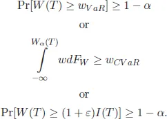
In addition to investment and consumption decisions being constrained by the available capital, the investor may have financial requirements or goals/targets to meet at the horizon such as:

Finally, there also may be limits placed on trading which constrain decisions, e.g., short selling and rebalancing.

The functions defining the decision model are presented in continuous time, but differencing and summation operators could replace the differential and integral. The richest formulations are discrete time stochastic dynamic models which are solved with multi-period stochastic programming (Ziemba, 2003). The continuous time models yield qualitative results which are useful for characterizing decision behavior.

The utility function is overconsumption at each time period and a bequest function of final wealth. Typically these functions are assumed to be concave risk averse. In the models presented in chapters included in this section, either U₀ ≡ 0 or U₁ ≡ 0.

The budget constraint defines the change in wealth from the returns on investment and the consumption at each time period. The returns have a diffusive process component (x′(α − re)+ r)W dt, and a point process (shock) component θ_tdN_t(λ_t). The diffusion is geometric Brownian motion (or a geometric random walk) and the point process is a type of Poisson process. An important feature of the point process is the dependence of the shock intensity on market conditions. This generates clusters of up/down shocks (Consigli et al. 2009). Alternatively, the ...

Table of contents

• Cover page
• Title
• Copyright
• Dedication
• Preface
• Contents
• Books for which the Problems are Designed
• Section A: Arbitrage and Asset Pricing
• Section B: Utility Theory
• Section C: Stochastic Dominance
• Section D: Risk Aversion and Static Portfolio Theory
• Section E: Risk Measures
• Section F: Dynamic Portfolio Theory and Asset Allocation
• About the Authors
• Index