![]()
Chapter 1
Samples and Selection Effects
1.1Introduction: which sample for which science goal?
1.1.1General rules to optimize the scientific returns from a survey of distant galaxies
The present-day generation of instruments allows us to study distant galaxies in considerable details. We can now determine the mass, dynamics, abundances, stellar population, and star formation efficiency of galaxies. While one could hope to learn a lot from previous work done in the local Universe, distant galaxies are unfortunately not like those in the local Universe both observationally (they are faint and small) and intrinsically (they are in principle less evolved).
To study how galaxies form and evolve, to test the curvature of the Universe or to investigate the epoch of reionization, astronomers rely on samples of galaxies for which they measure their redshifts, i.e., the so-called redshift surveys. While the redshift is assumed to be a fair indicator of the distance of a galaxy, there are many different criteria that can be used to select galaxies. One must therefore ensure that the selection criteria that were used are appropriate for the scientific objectives. For example, to study galaxy evolution one can study galaxy populations that are at different redshifts within the same redshift survey, or, alternatively, gather a comparison sample of galaxies at lower redshifts or in the Local Universe.
As was learned from the numerous redshift surveys, a simple, single, selection criterion such as apparent luminosity is preferred. This avoids having to deal with multiple selection effects that can cause some results to be very difficult to interpret, particularly with evolutionary studies. Even when using a single selection criterion for a redshift survey, one should carefully investigate possible biases that may prevent a representative analysis (see Ex. Introduction to the k-correction effects).
We will also discuss other means to select galaxies, using a color selection or photometric redshift techniques (see Sec. 1.5). These two selection techniques do not, however, provide true measurements of redshift1 and we therefore discuss these later. These methods are increasingly popular, especially when estimating the redshifts of distant galaxies which are often selected using similar spectral energy distribution based techniques (see Sec. 1.6).
Example 1.1: Introduction to the k-correction effects
It would be hard to test the evolution of elliptical galaxies up to z = 1.5 using a redshift survey based on the observed luminosity in a filter bluer than 800nm. This is because the luminosity of these galaxies drops abruptly below the 400nm (so-called 4000 Å) break. At z ≥ 1, such a selection will be principally driven by episodic star formation events dominated by UV luminous hot stars, and not by the bulk of the stellar mass. A very large k-correction is required when selecting z ≥ 1 galaxies in the rest-frame UV. This effect can result in an apparent lack of elliptical galaxies in the redshift survey since their UV emission is so faint. It is therefore essential to select objects at a restframe wavelength greater than 400nm (see Sec. 1.3.6).
Once a consistent method to select galaxies at a chosen redshift has been established, one should also prepare for additional observations that are needed to estimate additional physical quantities such as mass, abundances, stellar population, star formation. These additional measurements often need to be made at various wavelengths which bring additional selection effects, often caused by insufficient depth or resolution. For example, far-IR (FIR) observations of distant galaxies are often more limited in depth and spatial resolution than optical observations, i.e., detecting only the lower number density sub-sample of FIR-bright galaxies.
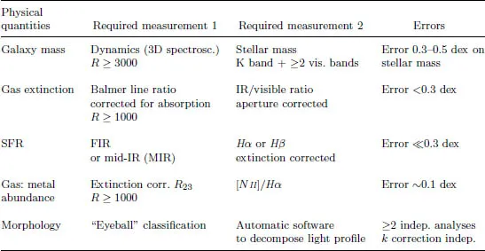
Table 1.1 illustrates how complementary observations can be used. It also shows how duplicating estimates at two different wavelengths can product a more robust estimate of a given physical quantity.
The way a galaxy sample is defined has considerable impact on the science that can be done with. It is a complex problem that must be handled carefully before any observations are attempted.
This chapter provides elementary guidelines that are based on common sense but it also tries to identify most of the usual pitfalls that can seriously affect studies of distant galaxies. It presents a logical sequence of problems encountered by scientific investigators aiming to assemble a sample of distant galaxies.
Section 1.2 describes the magnitude systems used along the book and presents general rules for estimating magnitudes. Section 1.3 shows how a galaxy sample can be obtained using imaging data, describing and providing solutions to the numerous problems linked to the photometric depth, to selection effects and biases, and to k-corrections. Section 1.4 describes how to prepare a galaxy redshift survey and how to derive the luminosity function (LF), and outlines the limitations of existing surveys and what can and cannot be derived from them. Section 1.5 presents an alternative way to estimate redshifts using photometry, and also explains why these photometric redshifts are not as robust distance measurements as spectroscopic redshifts. Section 1.6 deals specifically with very distant galaxies redshift surveys. Selecting these objects using photometry is difficult since they are overwhelmingly dominated in numbers by foreground galaxies. Section 1.7 describes techniques to identify a sample of distant galaxies that can be causally linked to nearby galaxies.
Table 1.1: Combination of measurements required for a robust determination of physical quantities of distant galaxies.
1.2General rules for estimating magnitudes
Before one can begin to understand the complexity of the selection effects present in distant galaxy samples, important steps needed to define the astronomical magnitude system must be clarified. The reader is encouraged to read Chapter 2 to learn the basic of photometric measurements and their uncertainties.
Several fundamental galaxy properties are directly related with luminosities in various bands. This includes the star formation rate (SFR) (combination of UV and mid to far IR luminosities), the stellar mass (which can be indirectly related to the near-infrared (NIR) luminosity), and bolometric luminosity. Special care must therefore be taken to measure magnitudes that are independent of the distance of a galaxy.
1.2.1Monochromatic and integrated magnitudes
Galaxies emit light over a wide range of order of magnitudes. It is therefore useful to use a logarithmic scale to quantify observed fluxes. Apparent magnitudes and fluxes are related following the classic Pogson relation:
where fν is the flux spectral density in erg/s/cm2/Hz, and ZP is the zero point used to set the origin of the logarithmic scale. In optical wavelengths, it is conventional to deal with spectral densities per wavelength unit rather than per frequency unit. Both quantities are related as follows:
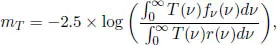
When fν is the average flux density over a spectral filter T, the magnitude is often written as mT, and is derived as follows:
where r(ν) is the monochromatic response of a reference source taken as zero point, and T(ν) is the filter transmission as a function of frequency (see, e.g., Sterken and Manfroid, 1992).
1.2.2Photometric systems
A photometric system is defined by a set of zero points defined at different wavelengths (or filters).
There are two commonly used photometric systems. Historically, people have used the Vega system, which uses the Vega star as a zero point in all filters. However, detectors have now become too sensitive to use Vega itself for calibration, and observing secondary standard stars is ...