Microeconomics With Spreadsheets

Suren Basov

• Publisher: WSPC
• Year: 2016
• eBook ISBN: 9789813143975
• Topic: Economía
• Subtopic: Teoría económica

Microeconomics studies the choices made by individuals under conditions of scarcity of resources and time and the interaction between different decision makers. Scarcity forces economic actors to choose one opportunity among many. Microeconomics with Spreadsheets starts with the mathematical preliminaries and covers consumer theory, producer theory, general equilibrium, game theory, market structure and economics of information.

The reader will use numerical tools to analyse problems that cannot be analysed analytically. There is a natural synergy between rigorous proofs and numerical methods, since before using a numerical method one should also prove that a solution exists and analyse whether it is unique, and therefore be able to interpret properly the output of a program.

0 Readership: Third year undergraduate and honours students along with postgraduate students taking advanced courses and modules on microeconomics.
Microeconomics, Game Theory, Producer Theory, Consumer Theory, Economics of Information, Basics of Industrial Organization, Excel, The Solver0

PART I

Mathematical Preliminaries

Overview

In this part, I am going to present the main mathematical tool that we will use during the course: constraint optimization. While presenting this material, I will assume that the students are familiar with calculus, matrix algebra, basic logic and set theoretic notations. However, for the reader not familiar with any of these techniques, they, together with some other techniques used in this course, are presented in the Mathematical Appendix in the last part of the book.

Chapter 1

Constraint Optimization

This chapter introduces reader to constraint optimization technique that is used through the book.

1.1 Constraint optimization with equality constraints

Often in economics, you are asked to maximize or minimize an objective function subject to some constraints. For example, consumers are assumed to maximize their utility given their budget and prices, firms often have to find an optimal way to produce a given quantity of products, which leads to minimizing cost of production taking the level of production, technology, and factor prices as given, etc. One can always turn a constraint minimization into a constraint maximization by changing the sign of the objective function. Therefore, we will formulate all results for constraint maximization problems. Ubiquity of constraint optimization problems in economics comes from the central assumption that economic agents act rationally in pursuing their self-interest. Main mathematical result that allows one to deal with the constraint optimization problems is summarized in the following theorem.

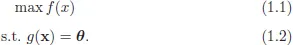
Theorem 1. Let f : X → R be a real-valued function and g : X → R^m be a mapping, where X ⊂ Rⁿ. Let us consider the following optimization problem:

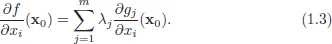
Assume that the solution is achieved at x₀ and vectors (∇g₁(x₀),...,∇g_m(x₀)) are linearly independent non-degenerate constraint qualifications (NDCQ). Then

Intuitively, if (1.3) does not hold, one can find point x₀ + δx such that

Recall that

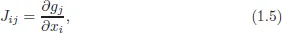
Therefore, for x₀ to be the optimum ∇f(x₀) · δx should be zero. Now, note that locally the surface g(x) = θ looks like a hyperplane and (∇g₁(x₀),...,∇g_m(x₀)) forms a basis (by NDCQ) in its orthogonal complement. Therefore,

for some λ₁,... , λ_m.

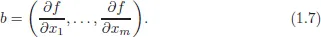
Proof. Note that NDCQ implies that m ≤ n. If m = n, then vectors (∇g₁(x₀),...,∇g_m(x₀)) form a basis in Rⁿ and expansion (1.4) can be found for any vector, including ∇f(x₀). Therefore, from now on, we will assume that m< n. NDCQ is equivalent to the statement that the Jacobian matrix J, defined by

has full rank at x₀. Therefore, it must have m independent rows. Without loss of generality, we will assume that first m rows of the Jacobian matrix, evaluated at x₀, are independent.¹ Therefore, Eq. (1.3) can be made to hold for

by choosing

where J_m is an m × m matrix formed by the first m rows of matrix J and

To prove that Eq. (1.3) also holds for

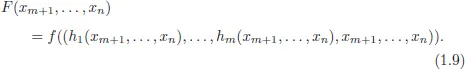
for the same choice of λ, recall that by the Implicit Function Theorem,² there exist a neighborhood³ U of point x₀ and continuously differentiable functions

,

such that

for all x ∈ U . Moreover,

where ∇_n−m denotes vector of partial derivatives with respect to variables

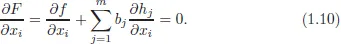
Note that x₀ delivers an unconstraint local maximum to function

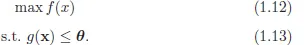
Using the first-order condition for unconstraint optimization and the chain rule, one can write the following:

Note that in matrix notation,

which completes the proof.

1.2 Constraint optimization with inequality constraints

Sometimes, relevant constraints are represented by inequalities rather than equalities. For example, a consumer may be offered a menu of choices. Relevant incentive constraints, which we will discuss later in this course, will specify that she should like the item designed for her at least as much as any other item on the menu. Generalization of the above theorem for the case of inequality constraints is given by the following theorem.

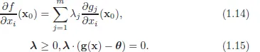
Theorem 2. Let f : X → R be a real-valued functional and g : X → R^m be a mapping, where X ⊂ Rⁿ. Let us consider the following optimization problem:

Assume that the solution is achieved at x₀ and vectors (∇g₁(x₀),...,∇g_m(x₀)) are linearly independent (NDCQ).Then

This statement is known as the Kunh–Tucker theorem. Intuitively, the first-order conditions state that the gradient of the objective function should look in a direction in which all the constraints are increasing, since otherwise one can move in a direction that will leave the choice variable x within the constraint set, but increase the value of the objective. I will not give the complete proof of this theorem. However, it is quite easy to see intuitively why it is true. Indeed, if a certain constraint does not...

Table of contents

• Cover Page
• Title
• Copyright
• Preface
• Author Biography
• Contents
• Part I Mathematical Preliminaries
• Part II Market Interactions
• Part III Strategic Interactions
• Part IV The Economics of Information
• Part V Mathematical Appendix
• Index