![]()
Part I
![]()
Chapter 1
Introduction
Shivom Sharma1 and Gade Pandu Rangaiah2,*
1Industrial Process and Energy Systems Engineering
École Polytechnique Fédérale de Lausanne,
CH-1951 Sion, Switzerland
2Department of Chemical and Biomolecular Engineering
National University of Singapore, 117585 Singapore
1.1Process Optimization
Optimization is an approach to find the best possible solution in the domain of interest while satisfying relevant constraints (restrictions). Optimization problems can be found everywhere, from engineering to economics and from daily life to holiday planning. For example, holiday planning optimization finds the place(s) to visit, when to visit, how to travel and duration of stay (which are all decision variables) to achieve the most happiness (which is the objective function or performance criterion); this may have constraints on budget, travel dates and places to visit as well as other objectives such as safety.
Optimization has been fruitfully applied to improve the performance and/or understanding in diverse areas such as science, engineering, business and economics. The goal of optimization is to find the values of decision variables, which will maximize or minimize the value of a given objective function (performance criterion) without violating specified constraints. Mathematically, an optimization problem can be stated as follows.
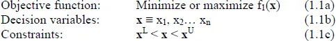
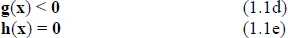
Here, f1(x) is the given objective function, x is the set of decision variables with xL and xU as the lower and upper bounds, and g and h are the set of inequality and equality constraints, respectively. Many application problems have more than one decision variable and a number of inequality and/or equality constraints.
An optimization problem is generally assumed to have only one objective function as in equation (1.1a); such problems belong to single-objective optimization (SOO). Each of these problems will have one or more optimal solutions. Note that optimization refers to both minimization and maximization, and an optimum can be either a minimum or a maximum. A minimization objective can be transformed into a maximization objective by multiplying with –1 or taking reciprocal (with a suitable modification to avoid division by zero). Similarly, a minimization method can easily be modified to a maximization method. Many books describe optimization for minimization, and we follow the same in this chapter. In other words, optimization and optimum are used as synonymous with minimization and minimum, respectively.
In the literature, numerous chemical engineering application problems have been optimized for single objective (e.g., see Himmelblau, 1972; Edgar et al., 2001; Ravindran et al., 2006; Rangaiah, 2010; Floudas, 2013). For example, optimization has been successfully applied in the design and operation of chemical and refinery processes, biotechnology, food technology, pharmaceuticals, fuel cells, power plants and bio-fuel production. Capital/equipment cost, operating cost, profit, net present value, energy consumption, efficiency, conversion, yield, selectivity, eco-indicator 99, global warming potential and CO2 emissions are the commonly used objective functions in process optimization problems.
1.2Classification of Optimization Methods
Optimization problems and methods can be classified in various ways using the characteristics summarized in Table 1.1. Some of these are briefly described in the following sub-sections. Many chemical engineering application problems have more than one variable and bounds on variables. Also, they often contain constraints arising from governing equations (such as mass and energy balances, and rate equations) and from process limitations (such as on maximum temperature, pressure and flow rate for safety and due to material of construction).
Table 1.1 Characteristics and classification of optimization problems and methods
| Characteristic | Classification |
| Number of variables: one or more | Single variable or multivariable optimization |
| Type of variables: real, integer or mixed | Nonlinear, integer or mixed (nonlinear) integer programming |
| Nature of equations: liner or nonlinear | Linear or nonlinear programming |
| Constraints: no constraints (besides bounds) or with constraints | Unconstrained or constrained optimization |
| Number of objectives: one or more | Single-objective or multi-objective optimization |
| Derivatives: without or using derivatives | Direct or gradient search optimization |
| Optimum: local or global in the search space | Local or global optimization |
| Random numbers: without or using random numbers | Deterministic or stochastic optimization methods |
| Trial points/solutions: one or more in each iteration | Single point (also known as trajectory) or population based methods |
1.2.1Use of derivatives
Optimization methods can be classified based on the use of derivate information. If the objective function and constraints are continuous and differentiable, then derivative-based methods such as steepest descent, quasi-Newton and successive quadratic programming (SQP) methods based on gradient vector can be used. These methods are computationally efficient, and give the same solution in different runs if the initial point is the same. Derivative-free methods (e.g., Nelder-Mead or downhill simplex) are used when the objective function or constraints have discontinuities. Both gradient-based and gradient-free methods can be used for solving SOO problems. Some of them are for unconstrained optimization whereas others for problems with constraints. For example, Nelder-Mead, steepest descent and quasi-Newton methods are for problems without constraints, whereas simplex, generalized reduced gradient (GRG) and SQP methods are for constrained optimization. For details on these methods, see Edgar et al. (2001) and Ravindran et al. (2006).
1.2.2Local and global methods
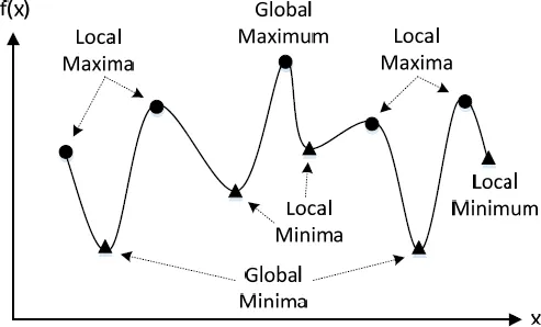
A given optimization problem may have more than one optimum. Fig. 1.1 illustrates this situation for both minima and maxima; in this figure, x-axis represents the search space in one or many decision variables, and the objective function (y-axis) can be for minimization or maximization. There are three local minima, two global minima, four local maxima and one global maximum in Fig. 1.1. By definition, a local minimum is the minimum in its nearby region whereas a global minimum is the lowest minimum over the entire search region (within bounds and satisfying constraints, if any). The objective function in Fig. 1.1 is neither convex nor concave over the entire region, and it is said to be multi-modal.
Fig. 1.1 Local and global optima of an optimization problem
Based on their search capability, optimization methods can be classified into local and global methods. Local search methods generally converge to an optimum in the neighborhood of the initial/starting point. Nelder-Mead, steepest descent, quasi-Newton, GRG and SQP methods are local search methods. These methods require an initial point or solution for starting the search, and converge to a nearby minimum, which can be local or global minimum. On the other hand, global methods search the entire search space, have the capability to escape from the local optimum and to find the global optimum. Multi-start is a simple strategy for searching global optimum using local methods in conjunction with a number of initial points. Global optimization methods, particularly stochastic methods, may not be successful in every run, and they need more computation time compared to local optimization methods. Randomization is an important component of stochastic search methods. There are many global methods, and they are introduced in the next sub-sections.
1.2.3Deterministic or stochastic methods
Optimization methods can also be classified into deterministic and stochastic methods. In deterministic optimization methods, the search for optimum is not random, i.e., it does not depend on random numbers; rather, the search is determined according to the algorithm, optimization problem and initial point. Hence, the new solution found in each iteration does not depend on random numbers. The final/converged solution by a deterministic method depends on the initial point. Examples of deterministic optimization methods are Nelder-Mead (also known as downhill simplex), steepest descent, quasi-Newton, GRG and SQP methods, which are all local methods. They are computationally efficient and can locate the optimum precisely. If the optimization problem is multi-modal as in Fig. 1.1, they are likely to converge to a local minimum near the initial point/solution, thus failing to find the global minimum. Note that deterministic methods require continuous and differentiable objective function and constraints.
Stochastic optimization methods, on the other hand, employ random numbers in their search strategies and are more likely to find the global optimum but they generally require more computational time and give less precise optimum compared to the deterministic methods. Almost all of them do not require continuity and differentiability of equations in the optimization problem as well as the initial/starting solution. Hence, stochastic methods can be applied to any type of optimization problems including black-box problems, wherein only the effect of decision variables on the objective and/or constraints is known (and not the underlying mathematical equations and their nature). Since they use random numbers in their search, they may converge to slightly different solutions in different runs. Stochastic optimization methods are based on search using a single point/solution or population of points/solutions, and they are inspired by logic, physical and/or natural phenomena. Simulated annealing (SA), genetic algorithms (GA), differential evolution (DE), particle swarm optimization (PSO) and ant colony optimization (ACO) are stochastic SOO methods. They are also known as metaheuristic...