Simulating Copulas: Stochastic Models, Sampling Algorithms, And Applications (Second Edition)

Stochastic Models, Sampling Algorithms, and Applications

Jan-Frederik Mai, Matthias Scherer;;;

• Publisher: WSPC
• Year: 2017
• Edition: 2
• eBook ISBN:
  9789813149267
• Topic: Mathematics
• Subtopic: Finance
• Index: Mathematics

-->

The book provides the background on simulating copulas and multivariate distributions in general. It unifies the scattered literature on the simulation of various families of copulas (elliptical, Archimedean, Marshall-Olkin type, etc.) as well as on different construction principles (factor models, pair-copula construction, etc.). The book is self-contained and unified in presentation and can be used as a textbook for graduate and advanced undergraduate students with a firm background in stochastics. Besides the theoretical foundation, ready-to-implement algorithms and many examples make the book a valuable tool for anyone who is applying the methodology.

--> Contents:

• Introduction
• Archimedean Copulas
• Marshall–Olkin Copulas
• Elliptical Copulas
• Pair Copula Constructions
• Sampling Univariate Random Variables
• The Monte Carlo Method
• Further Copula Families with Known Extendible Subclass
• Appendix: Supplemental Material

-->
--> Readership: Advanced undergraduate and graduate students in probability calculus and stochastics, practitioners who implement models in the financial industry and scientists. -->
Copula;Simulation;Monte Carlo;Random Vector;Dependence Model Key Features:

• Explicit focus on stochastic representations of copulas in contrast to an analytical perspective
• Easy-to-implement simulation schemes given as pseudo code
• Explicit focus on high-dimensional models
• Focus on applicability of models, e.g. to portfolio credit risk or insurance

Chapter 1

Introduction

Before we start, let us clarify some notations.

General comment: The dimension of a random vector is typically denoted by d ≥ 2.

Important sets: N denotes the set of natural numbers {1, 2, . . .}, and N₀ := {0} ∪ N. R denotes the set of real numbers. Moreover, for d ∈ N, R^d denotes the set of all d-dimensional row vectors with entries in R. For v := (v₁, . . . , v_d) ∈ R^d, we denote by v′ its transpose. For some set A, we denote by B(A) the corresponding Borel σ-algebra, which is generated by all open subsets of A. The cardinality of a set A is denoted by |A|. Subsets and proper subsets are denoted by A ⊂ B and A

B, respectively.

Probability spaces: A probability space is denoted by (Ω, F, P), with σ-algebra F and probability measure P. The corresponding expectation operator is denoted by E. The variance, covariance, and correlation operators are written as Var, Cov, Corr, respectively. Random variables (or vectors) are mostly denoted by the letter X (respectively X := (X₁, . . . , X_d)). As an exception, we write U := (U₁, . . . , U_d) for a d-dimensional random vector with a copula as joint distribution function.¹ If two random variables X₁, X₂ are equal in distribution, we write X₁

X₂. Similarly,

denotes convergence in distribution. Elements of the space Ω, usually denoted by ω, are almost always omitted as arguments of random variables, i.e. instead of writing X(ω), we simply write X. Finally, the acronym i.i.d. stands for “independent and identically distributed”.

Functions: Univariate as well as d-dimensional distribution functions are denoted by capital letters, mostly F or G. Their corresponding survival functions are denoted

,

. As an exception, a copula is denoted by the letter C; its arguments are denoted (u₁, . . . , u_d) ∈ [0, 1]^d. The characteristic function of a random variable X is denoted by ϕ_X(x) := E[exp(ixX)]. The Laplace transform of a non-negative random variable X is denoted by φ_X(x) := E[exp(−xX)]. Moreover, the nth derivative of a real-valued function f is abbreviated as f⁽ⁿ⁾; for the first derivative we also write f′. The natural logarithm is denoted log.

Stochastic processes: A stochastic process X : Ω × [0, ∞) → R on a probability space (Ω, F, P) is denoted by X = {X_t}_t≥0, i.e. we omit the argument ω ∈ Ω. The time argument t is written as a subindex, i.e. X_t instead of X(t). This is in order to avoid confusion with deterministic functions f, whose arguments are written in brackets, i.e. f(x).

Important univariate distributions: Some frequently used probability distributions are introduced here. Sampling univariate random variables is discussed in Chapter 6.

(1)U[a, b] denotes the uniform distribution on [a, b] for −∞ < a < b < ∞. Its density is given by f(x) =

_{x∈[a,b]} (b − a)⁻¹ for x ∈ R.

(2)Exp(λ) denotes the exponential distribution with parameter λ > 0, i.e. with density f(x) = λ exp(−λx)

_{x>0} for x ∈ R.

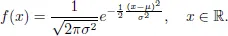
(3)N(µ, σ²) denotes the normal distribution with mean µ ∈ R and variance σ² > 0. Its density is given by

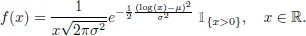
(4)LN(µ, σ²) denotes the lognormal distribution. Its density is given by

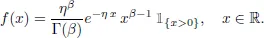
(5)Γ(β, η) denotes the Gamma distribution with parameters β, η > 0, i.e. with density

Note in particular that the expo...

Table of contents

• Cover
• Halftitle
• Series Editors
• Title
• Copyright
• Dedication
• Preface
• Contents
• 1. Introduction
• 2. Archimedean Copulas
• 3. Marshall–Olkin Copulas
• 4. Elliptical Copulas
• 5. Pair Copula Constructions
• 6. Sampling Univariate Random Variables
• 7. The Monte Carlo Method
• 8. Further Copula Families with Known Extendible Subclass
• Appendix A Supplemental Material
• Bibliography
• Index