Stock Market Crashes

Predictable and Unpredictable and What to do About Them

William T Ziemba, Mikhail Zhitlukhin;Sebastien Lleo;;

• Publisher: WSPC
• Year: 2017
• Topic: Economics
• eBook ISBN:
  9789813223868
• Subtopic: Finance
• Index: Economics

-->

This book presents studies of stock market crashes big and small that occur from bubbles bursting or other reasons. By a bubble we mean that prices are rising just because they are rising and that prices exceed fundamental values. A bubble can be a large rise in prices followed by a steep fall. The focus is on determining if a bubble actually exists, on models to predict stock market declines in bubble-like markets and exit strategies from these bubble-like markets. We list historical great bubbles of various markets over hundreds of years.

We present four models that have been successful in predicting large stock market declines of ten percent plus that average about minus twenty-five percent. The bond stock earnings yield difference model was based on the 1987 US crash where the S&P 500 futures fell 29% in one day. The model is based on earnings yields relative to interest rates. When interest rates become too high relative to earnings, there almost always is a decline in four to twelve months. The initial out of sample test was on the Japanese stock market from 1948-88. There all twelve danger signals produced correct decline signals. But there were eight other ten percent plus declines that occurred for other reasons. Then the model called the 1990 Japan huge -56% decline. We show various later applications of the model to US stock declines such as in 2000 and 2007 and to the Chinese stock market. We also compare the model with high price earnings decline predictions over a sixty year period in the US. We show that over twenty year periods that have high returns they all start with low price earnings ratios and end with high ratios. High price earnings models have predictive value and the BSEYD models predict even better. Other large decline prediction models are call option prices exceeding put prices, Warren Buffett's value of the stock market to the value of the economy adjusted using BSEYD ideas and the value of Sotheby's stock. Investors expect more declines than actually occur. We present research on the positive effects of FOMC meetings and small cap dominance with Democratic Presidents. Marty Zweig was a wall street legend while he was alive. We discuss his methods for stock market predictability using momentum and FED actions. These helped him become the leading analyst and we show that his ideas still give useful predictions in 2016-2017. We study small declines in the five to fifteen percent range that are either not expected or are expected but when is not clear. For these we present methods to deal with these situations.

The last four January-February 2016, Brexit, Trump and French elections are analzyed using simple volatility-S&P 500 graphs. Another very important issue is can you exit bubble-like markets at favorable prices. We use a stopping rule model that gives very good exit results. This is applied successfully to Apple computer stock in 2012, the Nasdaq 100 in 2000, the Japanese stock and golf course membership prices, the US stock market in 1929 and 1987 and other markets. We also show how to incorporate predictive models into stochastic investment models.

--> Contents:

• Introduction
• Discovery of the Bond–Stock Earnings Yield Differential Model
• Prediction of the 2007–2009 Stock Market Crashes in the US, China and Iceland
• The High Price–Earnings Stock Market Danger Approach of Campbell and Shiller versus the BSEYD Model
• Other Prediction Models for the Big Crashes Averaging –25%
• Effect of Fed Meetings and Small-Cap Dominance
• Using Zweig's Monetary and Momentum Models in the Modern Era
• Analysis and Possible Prediction of Declines in the –5% to –15% Range
• A Stopping Rule Model for Exiting Bubble-like Markets with Applications
• A Simple Procedure to Incorporate Predictive Models in Stochastic Investment Models
• Appendices:
  • Other Bubble-testing Methodologies and Historical Bubbles
  • Mathematics of the Changepoint Detection Model

-->
--> Readership: Students, researchers and the general public who are interested to understand more about stock market crashes and what to do about them. -->
Keywords:Stock Market Crashes;Brexit;Trump;Financial BubblesReview:0

Chapter 1

Introduction

Trying to predict stock market declines or crashes is important to all investors and especially to speculative investors and hedge funds. Avoiding them or dealing with them greatly improves portfolio performance. But it is hard to predict these declines. Moreover, to quote Peter Lynch:

Far more money has been lost by investors preparing for corrections, or trying to anticipate corrections, than has been lost in corrections themselves.

Financial bubbles and crashes are certainly not new, and the most dramatic ones tend to leave a lasting memory. “The South Sea Bubble, a Scene in ‘Change Alley in 1720’,” reproduced in Figure 1.1, was painted by Edward Matthew Ward in 1847, nearly 130 years after the events but only a couple of years after another famous stock market bubble: Railway Mania.¹

The academic literature on bubbles and crashes is well established, starting with the studies on bubbles by Blanchard and Watson (1982), Flood et al. (1986), Camerer (1989), Allen and Gorton (1993), Diba and Gross-man (1988), Abreu and Brunnermeier (2003) and more recently Corgnet et al. (2015), Andrade et al. (2016) or Sato (2016). A rich literature on bubble and crash predictions has also emerged. We can classify most bubble and crash prediction models in three broad categories based on the type of methodology and variable used: fundamental models, stochastic models and sentiment-based models.

Fundamental models use fundamental variables such as stock prices, corporate earnings, interest rates, inflation or GNP to forecast crashes. The bond–stock earnings yield differential (BSEYD) measure (Ziemba and Schwartz, 1991; Lleo and Ziemba, 2012, 2015c, 2017) is the oldest model in this category, which also includes the CAPE (Lleo and Ziemba, 2017) and the ratio of the market value of all publicly traded stocks to the current level of the GNP (MV/GNP) that Warren Buffett popularized (Buffett and Loomis, 1999, 2001; Lleo and Ziemba, 2016b). Recently, Callen and Fang (2015) also found evidence that short interest is positively related to one-year ahead stock price crash risk.

Fig. 1.1. “The South Sea Bubble, a Scene in ‘Change Alley in 1720’ ” by Edward Matthew Ward (1816–1879).

Stochastic models construct a probabilistic representation of the asset prices. This representation can be either a discrete or a continuous time stochastic process. Examples include the local martingale model proposed by Jarrow and Protter (Jarrow et al., 2010, 2011; Jarrow and Larsson, 2012; Protter, 2013; Jarrow, 2016; Protter, 2016), the disorder detection model proposed by Shiryaev, Zhitlukhin and Ziemba (Shiryaev, 2010a; Shiryaev et al., 2014, 2015) and the earthquake model of Gresnigt et al. (2015). When it comes to actual implementation, the local martingale model and the disorder detection model share the same starting point: they assume that the evolution of the asset price S(t) can be best described using a diffusion process:

where W (t) is a standard Brownian motion on the underlying probability space. However, the two models look at different aspects of the evolution. The disorder detection model detects crashes by looking for a change in regime in the drift µ and volatility σ. The local martingale model detects bubbles by testing whether the process is a martingale or a strict local martingale.

Behavioral analyses, such as the recent work by Goetzmann et al. (2016), are the latest addition to the bubble and crash literature. The emphasis here is on the way individuals assess the probabilities of market crashes, and on the discrepancy between these subjective probability and the historical probabilities observed on the market.

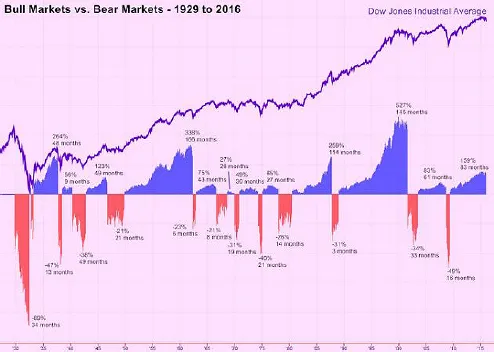
In this book, we present models that have been shown to predict many large crashes averaging −25%. We also discuss how to deal with small declines in the −5% to −15% range. The S&P500 had 22 10%+ corrections over less than a year since the mid-1960s. Figure 1.2 shows the cycles of bull and bear markets on the Dow Jones Industrial Average (DJIA) from 1929 to 2016. In China, the Shanghai Composite Index had 22 such corrections since it opened 25 years ago, and the Shenzhen Composite Index, 21.

Fig. 1.2. Bull and Bear Markets on the Dow Jones Industrial Average (1929–2016).

Source: Yahoo!

The discussion proceeds by discussing when a bubble exists. A bubble exists when prices are trending just because they are trending up or down. The definition and identification of whether a particular market is a bubble or not is complex and is discussed in Appendix A.

1.1.How rare are bubbles?

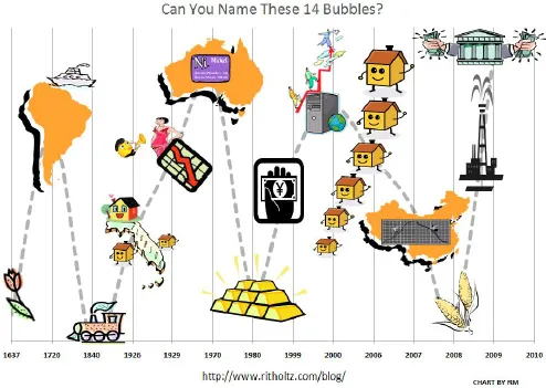
In this book, we present evidence associated with trying to predict when a bubble exists, when it might burst and deflate and how to get out of bubble-like markets near the top. From Tulip Mania to the Mississippi Bubble, the South Sea Bubble. The 1929 Crash, the dotcom bubble and the housing bubble. Figure 1.3 is a visual reminder that bubbles and crashes have occured for a long time, all around the world. Goetzman in (2014) considers the questions on how rare are these bubbles and what happens to them. When they burst do they give back most or all of the gain in their rise to bubble status?

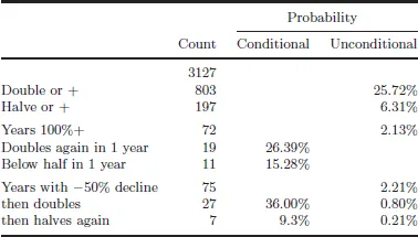
Goetzmann, using the 1900–2014, 21-country world equity market data from Dimson et al. (2014), found that bubbles are quite rare, the chance that a market that doubles gives back its gain is only about 10%, markets are more likely to double again following a 100% doubling move, and that the probability of a crash conditional on a bubble-like boom is only slightly higher than the unconditional probability., namely 0.3–1.4% for various bubble definitions.

Fig. 1.3. Around the world in 14 crashes.

Goetzmann defines a boom as a 100% increase in (a) one year or (b) three years and defines a crash or drop of at least 50% (a) in the next year or (b) in the next five years. To be specific in 3470 market years there were 72 one year returns of 100%+ and 84 with returns less than −50% busts. Of the 72 booms, 6 (8.33%) doubled again versus an unconditional frequency of 0.18%, and 3 (4.1%) fell by a half or more versus an unconditional 0.09%. And of the 84 busts, 10 (13.16%) doubled versus 0.3% unconditional and 5 (0.50%) halved again versus 0.15% unconditional.

Over five years, there are a lot more doubling gains and halving loses. The results are in Table 1.1.

1.2.How many crashes and how deep are they going to be in the opinion of investors?

The data show that single-day large drops in equity prices are rare. But we have some large ones such as October 28, 1929, October 19, 1987 and September 11, 2001. These all occurred during a period of high volatility with prices rising and falling dramatically in the period before the big drop day. Table 1.2 lists the 10 largest 1-day declines in the S&P500 from 1928 to 2016. One sees many large drops in october. Also, only three days had declines greater than 10%.

Table 1.1. Five year doubling and halving results.

Source: Goetzmann (2014).

Table 1.2. The 10 largest 1-day declines in the S&P500.

LARGEST ONE DAY DROPS EVER FOR THE S&P500. OCTOBER IS WELL REPRESENTED
Date	S&P500	Change
19/10/87	224.84	−20.5%
28/10/29	22.74	− 12.9%
29/10/29	20.43	− 10.2%
5/11/29	20.61	− 9.9%
18/10/37	10.76	− 9.1%
5/10/31	8.82	− 9.1%
15/10/08	907.84	− 9.0%
1/12/08	816.21	− 8.9%
20/7/33	16.57	− 8.9%
29/9/08	1106.39	−8.8%

Source: UPI Research FactSet 11/10/16.

Goetzmann et al. (2016) show with surveys of high net worth individual and institutional investors over 26 years in the US 1989–2015 that these investors expect many more crashes than actually occur. They found that recent market declines and adverse market events and media reporting boost these probabilities. They also found that non-market related rare disasters yield higher investor subjective crash probabilities. The following question is asked:

What do you think is the probability of a catastrophic stock market crash in the US like that of October 28, 1929 or October 19, 1987, in the next six months, including the case that a crash occurred in the other countries and spreads to the US? (An answer of 0% means that it cannot happen, an answer of 100% means it is sure to happen.
Probability = ______ %.)

The mean and median responses were an astounding 19% and 10%, respectively, about 10 times the actual frequency which was about 1.7% over the period October 23, 1925 to December 31, 2015.

Chapter 2 discusses the bond-stock earnings yield differential model (BSEYD) model which Ziemba devised in Japan in 1988 based on the 1987 US stock market crash. In the model, we use the long bond rate versus the earning yield which is the reciprocal of the trailing price earnings (P/E)–ratio. When the difference is too high, a crash almost always occurs. By a crash, we mean a decline of 10% plus from the signal point within one year. We apply this to many markets including Japan and the US over a long period of time. Usually, the market rallies for a while past the signal date and then declines. The model has predicted many crashes. It also predicted two crashes where famed bubble George Soros shorted too soon and lost billions. The so-called FED model is the special case of the BSYED model when the difference between the long bond and the earnings yield on equities is zero.

In Chapter 3, we focus on the short window 2006–2009 crash period. The BSEYD model predicted the stock market crashes in Iceland which fell 95%, China where the market had a huge rally then fell below the signal point and the US which had a correct call on June 14, 2007 with the market falling from the 1500s to 666 in March 2009.

•Graphs show what happened. The US call was on June 14, 2007 with the S&P500 over 1500. Then it fell to 666 in early March 2009. Then a huge bull market more than tripled the S&P500, which is still going. We have simple graphs where two curves cross and one can be made a horizontal line for easy understanding.

•Ziemba was in Iceland in 2006 and the model was not in the danger zone for the index which is mostly banks acting as hedge funds. Small ...

Table of contents

• Cover
• Halftitle
• Series Editors
• Title
• Copyright
• Review Quotes
• Dedication
• Preface
• About the Authors
• Contents
• 1. Introduction
• 2. Discovery of the Bond–Stock Earnings Yield Differential Model
• 3. Prediction of the 2007–2009 Stock Market Crashes in the US, China and Iceland
• 4. The High Price–Earnings Stock Market Danger Approach of Campbell and Shiller versus the BSEYD Model
• 5. Other Prediction Models for the Big Crashes Averaging−25%
• 6. Effect of Fed Meetings and Small-Cap Dominance
• 7. Using Zweig’s Monetary and Momentum Models in the Modern Era
• 8. Analysis and Possible Prediction of Declines in the −5% to −15% Range
• 9. A Stopping Rule Model for Exiting Bubble-like Markets with Applications
• 10. A Simple Procedure to Incorporate Predictive Models in Stochastic Investment Models
• Appendix A. Other Bubble-testing Methodologies and Historical Bubbles
• Appendix B. Mathematics of the Changepoint Detection Model
• Bibliography
• Index