Advanced Finance Theories

Ser-Huang Poon

• Publisher: WSPC
• Year: 2018
• Topic: Mathematics
• eBook ISBN:
  9789814460392
• Subtopic: Corporate Finance
• Index: Mathematics

-->

For PhD finance courses in business schools, there is equal emphasis placed on mathematical rigour as well as economic reasoning. Advanced Finance Theories provides modern treatments to five key areas of finance theories in Merton's collection of continuous time work, viz. portfolio selection and capital market theory, optimum consumption and intertemporal portfolio selection, option pricing theory, contingent claim analysis of corporate finance, intertemporal CAPM, and complete market general equilibrium. Where appropriate, lectures notes are supplemented by other classical text such as Ingersoll (1987) and materials on stochastic calculus.

-->
--> Contents:

• Utility Theory
• Pricing Kernel and Stochastic Discount Factor
• Risk Measures
• Consumption and Portfolio Selection
• Optimum Demand and Mutual Fund Theorem
• Mean–Variance Frontier
• Solving Black–Scholes with Fourier Transform
• Capital Structure Theory
• General Equilibrium
• Discontinuity in Continuous Time
• Spanning and Capital Market Theories

-->
--> Readership: Graduates, doctoral students, researchers, academic and professionals in theoretical financial modeling in mainstream finance or derivative securities. -->
Keywords:Intertemporal Portfolio Selection;Capital Structure;General Equilibrium;Spanning;Mutual Fund Theorem;Jumps;Incomplete MarketsReview: Key Features:

• Complete and explicit exposition of classical finance theories core to theoretical finance research
• Modern treatments to some derivations
• Supplementary coverage on key related publications and more recent finance research questions
• Detailed proofs and explicit coverage to aid understanding by first year PhD students
• List of exercises with suggested solutions

Chapter 1

Utility Theory

This chapter derives asset prices in a one-period model. We derive a version of the Capital Asset Pricing Model (CAPM) using a complete market, state-contingent claims approach. We define the forward pricing kernel and then use the assumption of joint normality of the cash flows and Stein’s lemma to establish the CAPM. We then derive the pricing kernel in an equilibrium representative investor model. But first, we need to understand a few properties of utility function.

A common utility function we use in economics/finance is the power utility. Its functional form is:

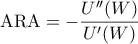
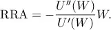
This may seem a strange choice for a utility functional form, but it is actually a very clever one. The Arrow–Pratt measures of (absolute and relative) risk aversion (RA) are

and

By the assumption of a risk averse investor, U(W) is increasing and strictly concave

The inverse of RA −

is also known as risk tolerance.¹

Using the power utility function, we get U′(W) = W^−γ and U′′(W) = −γW^−γ−1. Therefore, the Arrow–Pratt measure of Relative Risk Aversion (RRA) under power utility is RRA = γ. If γ > 0, then the agent is risk averse. If γ < 0, we would call her risk seeker (or lover). To satisfy the second common assumption of concavity, we need γ > 0. In other words, power utility function with γ > 0 refers to an investor with RRA that is independent of her level of wealth, which is why it is also called the constant RRA utility function.

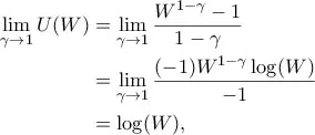
In the case where γ = 1 we get a special utility function, called the logarithmic function, U(W) = log(W). You can see that by taking the limit

after applying l’ Hôpital’s rule. Essentially, log utility function is a CRRA utility function with RRA = 1.

Another commonly used utility function is the negative exponential utility

so ARA = η and RRA = ηW. This is why this utility function is called the Constant Absolute Relative Risk Aversion (CARA) utility function. For an investor to be risk averse, we would require η > 0.

Finally, a linear utility function of the form U(W) = a + bW, corresponds to a risk-neutral investor. Why? Because U^′(W) = b and U^′′(W) = 0. In other words, the function is not concave (obviously, since it is linear in W) and the Arrow–Pratt measures of risk aversion are ARA = RRA = 0.

1.1Risk Aversion and Certainty Equivalent

For a given utility function U(⋅) and uncertain terminal wealth W, we can write W in terms of its certainty equivalent W_c as follows:

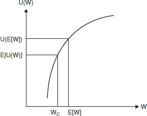
The term “risk averse” as applied to investors with strictly concave utility functions is descriptive in the sense that thecertainty-equivalent end-of-period wealth is always less than the expected value E(W) of the associated portfolio for all such investors. The proof follows from Jensen’s inequality: if U is strictly concave, then

The smaller the W_c, the more risk averse is the investor.

An investor is said to be more risk averse than a second investor if, for every portfolio, the certainty-equivalent end-of-period wealth for the first investor is less than or equal to the certainty equivalent end-of-period wealth associated with the same portfolio for the second investor. This statement is always true disregarding the shape of the risky return distribution and the order of risk preference.

¹Indeed, with the advances of research, we now know that these lower order of risk preference measures are not sufficient in distinguishing risks represented by higher moments of the risky return distribution. But we will confine our scope here to the classical analyses only omitting e.g. skewness preference.

Chapter 2

Pricing Kernel and Stochastic Discount Factor

2.1Arrow–Debreu State Prices

We assume that there are a finite number of states of the world at time t+T, indexed by i = 1, 2, . . . , I, each with a positive probability of occurring. Let p_i be the probability of state i occurring. A state-contingent claim on state i is defined as a security which pays $1 if and only if state i occurs.

We now assume that markets are complete. Specifically, we assume that it is possible to buy a state-contingent claim with a forward price q_i for state i. In complete markets, the q_i prices exist, for all states i. It follows that an asset j, which has a t...

Table of contents

• Cover
• Halftitle
• Title
• Copyright
• Dedication
• Preface
• About the Author
• Acknowledgements
• Contents
• Note for PhD Students
• 1 Utility Theory
• 2 Pricing Kernel and Stochastic Discount Factor
• 3 Risk Measures
• 4 Consumption and Portfolio Selection
• 5 Optimum Demand and Mutual Fund Theorem
• 6 Mean–Variance Frontier
• 7 Solving Black–Scholes with Fourier Transform
• 8 Capital Structure Theory
• 9 General Equilibrium
• 10 Discontinuity in Continuous Time
• 11 Spanning and Capital Market Theories
• Bibliography
• Calculus Notes
• Index