Applied Theoretical Organic Chemistry

Dean J Tantillo

• Publisher: WSPC (EUROPE)
• Year: 2018
• ISBN:
  9781786344106
• Topic: Physical Sciences
• Subtopic: Chemistry
• Index: Chemistry

-->

This book provides state-of-the-art information on how studies in applied theoretical organic chemistry are conducted. It highlights the many approaches and tools available to those interested in using computational chemistry to predict and rationalize structures and reactivity of organic molecules. Chapters not only describe theoretical techniques in detail, but also describe recent applications and offer practical advice.

Authored by many of the world leaders in the field of applied theoretical chemistry, this book is perfect for both practitioners of computational chemistry and synthetic and mechanistic organic chemists curious about applying computational techniques to their research.

--> Contents:

• Modeling Organic Reactions — General Approaches, Caveats, and Concerns (Stephanie R Hare, Brandi M Hudson and Dean J Tantillo)
• Overview of Computational Methods for Organic Chemists (Edyta M Greer and Kitae Kwon)
• Brief History of Applied Theoretical Organic Chemistry (Steven M Bachrach)
• >
• Solvation (Carlos Silva Lopez and Olalla Nieto Faza)
• Conformational Searching for Complex, Flexible Molecules (Alexander C Brueckner, O Maduka Ogba, Kevin M Snyder, H Camille Richardson and Paul Ha-Yeon Cheong)
• NMR Prediction (Kelvin E Jackson and Robert S Paton)
• Energy Decomposition Analysis and Related Methods (Israel Fernández)
• Systems with Extensive Delocalization (L Zoppi and K K Baldridge)
• Modern Treatments of Aromaticity (Judy I-Chia Wu)
• Weak Intermolecular Interactions (Rajat Maji and Steven E Wheeler)
• Predicting Reaction Pathways from Reactants (Romain Ramozzi, W M C Sameera and Keiji Morokuma)
• Unusual Potential Energy Surfaces and Nonstatistical Dynamic Effects (Charles Doubleday)
• The Distortion/Interaction Model for Analysis of Activation Energies of Organic Reactions (K N Houk, Fang Liu, Yun-Fang Yang and Xin Hong)
• Spreadsheet-Based Computational Predictions of Isotope Effects (O Maduka Ogba, John D Thoburn and Daniel J O'Leary)
• Stereoelectronic Effects: Analysis by Computational and Theoretical Methods (Gabriel dos Passos Gomes and Igor Alabugin)
• p K a Prediction (Yijie Niu and Jeehiun K Lee)
• Issues Particular to Organometallic Reactions (Gang Lu, Huiling Shao, Humair Omer and Peng Liu)
• Computationally Modeling Nonadiabatic Dynamics and Surface Crossings in Organic Photoreactions (Arthur Winter)
• Challenges in Predicting Stereoselectivity (Elizabeth H Krenske)

-->
--> Readership: Practitioners of computational chemistry and synthetic and mechanistic organic chemists curious about applying computational techniques to their research. -->
Keywords:Organic Chemistry;Theoretical Chemistry;Stereoselectivity;NMR Prediction;pKa Prediction;Organic PhotoreactionsReview: Key Features:

• A particular strength is the mix of theoretical background, informative examples and practical advice provided
• Chapters are authored by many of world leaders in the field of applied theoretical chemistry

Chapter 1

Modeling Organic Reactions — General Approaches, Caveats, and Concerns

Stephanie R. Hare, Brandi M. Hudson and Dean J. Tantillo

Department of Chemistry, University of California — Davis, Davis, CA, USA

1.1Introduction

Computational chemistry is unique in that the researcher who uses it as a tool is not bound by the confines of reality. This freedom has both benefits and drawbacks because it not only allows the researcher to be boundlessly creative in determining how to answer chemical questions but also requires an understanding of all the assumptions being made in the analysis (which is often nontrivial). This chapter aims to describe the basics of applying quantum chemistry to organic structures and reactions and to highlight “everything that can go wrong” in quantum chemical calculations — that is, when the assumptions break down or are incorrectly applied.

1.1.1What can the Schrödinger equation do for YOU?

The primary goal of any quantum chemical computation is to associate an energy value with a particular distribution of electrons around nuclei in particular positions. This goal is achieved using the Schrödinger equation, shown below in its least threatening form (physically oriented chemists, please forgive):

In this equation, a distribution of electrons/electron density, expressed as a wave function (Ψ) is associated with an energy (E) by a Hamiltonian operator (H; an operator is a function that acts on another function). The Hamiltonian (for short), also the “functional” in density functional theory (DFT), is a function that contains terms associating energy values with the relative positions of electrons and nuclei (see Chapter 2 for a survey of different Hamiltonians). The Hamiltonian is also referred to as the “model chemistry”.

1.1.2Putting the Schrödinger equation to work

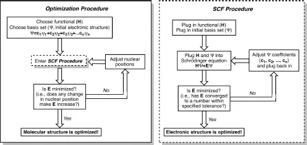
How is the Schrödinger equation used to predict a distribution of electrons/electron density? Generally, a prediction is arrived at by using the following procedure. (1) A basis set of atomic orbitals (usually Gaussian functions) is used by the quantum chemistry software of choice to construct guesses at the shapes (mathematical forms) of molecular orbitals (MOs). This step corresponds to the famous linear combination of atomic orbitals (LCAO) technique. In this step, electrons localized on individual atoms are transformed into electrons delocalized over molecules (or portions thereof). Note that basis sets are not restricted to one 1s, one 2s, three 2p orbitals, etc.; for example, many p-orbitals of differing “shapes” (e.g., short and squat, tall and diffuse) are generally used. By doing so, electrons are allowed to more freely explore larger regions of the space around the nuclei, thereby increasing their chances of finding ideal positions/distributions. While this all sounds rosy, the user is limited by the computational time required to perform such sampling, which is proportional (generally not linearly) to the number of basis functions used. (2) Once one has a guess at the MOs, the Hamiltonian then operates on the corresponding wave function that describes this orbital arrangement to calculate its energy. (3) Steps 1 and 2 are then repeated, changing the coefficients in the LCAO each time to produce different MOs and associated wave function, and correspondingly, a different energy. This iterative procedure (called the self-consistent field (SCF) procedure) continues until the energy is minimized (given particular convergence criteria built into the quantum chemistry software or set by the user). At the end, one has the “best” (lowest energy) distribution of electrons/electron density (wave function) for the given set of atomic/nuclear coordinates. From the wave function, myriad useful properties can be derived, e.g., spin densities, charge distributions, and NMR chemical shifts. As a whole, this calculation is called a single point calculation, since only one molecular geometry was considered.

1.1.3But what is the shape of the molecule?

If the user would also like to optimize relative atomic positions for the structure in question, i.e., derive ideal bond lengths, angles, and dihedral angles, then geometry optimization is carried out. This procedure involves a series of single point calculations. After carrying out the single point calculation on the initial geometry, the relative atomic (i.e., nuclear) coordinates are varied slightly, a new single point calculation is carried out and the energies associated with the old and new structures are compared. This goes on and on until a geometry is found with the lowest possible energy (Fig. 1.1). Thus, the optimization of electron positions/distributions is decoupled from the optimization of nuclear positions — which is allowed by the Born–Oppenheimer approximation, which notes that electrons move/adjust their positions much more quickly than do nuclei, because the former have much smaller masses than do the latter.

What control does the user possess over this process? First, the user must specify the Hamiltonian, e.g., HF, MP2, B3LYP, etc. (see Chapter 2). The Hamiltonian to be used in a particular calculation is generally determined on the basis of: (1) past experience (of the user or others, as reported in the literature) in applying particular Hamiltonians to molecules with particular functional groups and particular types of reactions and/or (2) test calculations in which the performance of particular Hamiltonians is assessed against experimental data or data from “high level” calculations (on small model systems, since such “high levels” are usually prohibitively expensive for organic molecules of sizes relevant to organic synthesis, bioorganic chemistry, etc.). Second, the user must specify the basis set. Again, this choice is generally made on the basis of precedent or model calculations. Some functional/basis set combinations are better than others for calculating the geometry of a molecule, while some are better than others for calculating the energy of a molecule. Third, the user must specify the initial atomic (nuclear) coordinates of the system to be studied. These coordinates are generally obtained from X-ray structures (on the off-chance that one is available) or result from the user’s chemical intuition piped through (nowadays) a graphical user interface attached to the quantum chemistry software of choice. If one is performing a geometry optimization, then the closer the initial geometry is to the optimized geometry the faster the calculation will be, i.e., there is a direct pay-off for having well-developed chemical intuition.

Figure 1.1.A flowchart showing the process by which quantum chemical software calculates the electronic structure and optimizes the geometry of a molecule. The SCF procedure occurs at each iteration of a geometry optimization to calculate the energy of the electronic structure of each nuclear geometry.

1.2Energy

Let us talk about the energy that is calculated in the procedure described above. Arguments regarding the reactivity of organic molecules almost always boil down to energy. There are various forms of energy that can be calculated using computational methods, with each step of a calculation bearing its own assumptions. Here we will briefly discuss how each type of energy is calculated and what major assumptions an applied theoretical chemist should know about to make valid arguments about a molecule’s reactivity. For a more detailed mathematical description of these calculations, specifically as they are implemented in the Gaussian program package, see the white papers by Frisch et al. and Ochterski et al.¹ on quantum chemistry and thermochemistry in Gaussian.

1.2.1Potential energy surfaces and stationary points

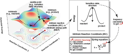
We will focus first on geometry optimization. The electronic energy (E), also called the potential energy, is the only type of energy calculated in a simple geometry optimization. This is the energy of all nuclei and electrons combined into a molecule (or complex) compared to the energy of all nuclei and electrons at infinite separation. Optimized molecular geometries correspond to points on a calculated potential energy surface (PES; Fig. 1.2). A PES describes how the energy of a molecule changes with changes in its geometry (i.e., nuclear positions and accompanying electron distribution). A molecular structure can be optimized to either a minimum (corresponding to a reactant, intermediate, or product) or first-order saddle point (a minimum with respect to all geometric changes except those that occur along the intrinsic reaction coordinate [IRC, vide infra], corresponding to a transition state structure [TSS]). Both minima and TSSs are “stationary points” on the PES, because the slope of the tangent to the surface at these points is zero. There has been some debate over the years about the terms “transition state,” “transition structure,” and “transition state structure.” We employ the convention that “transition structure” and “transition state structure” are synonyms, meaning a first-order saddle point on the PES, i.e., the high energy point along a particular optimized reaction coordinate. However, we reserve the term “transition state” for describing an ensemble of structures around a TSS, i.e., it is a state not a single structure. Transition states are particularly relevant in dynamics calculations (see Chapter 12).

Figure 1.2.A theoretical 3D PES (left) showing two minima and the TSS connecting them. The minimum energy pathway (MEP) between two minima is called the IRC, which has the 2D form shown on the right. A frequency calculation at each stationary point (minima and TSS) leads to calculation of the free energy barrier, which can be used in the Eyring equation² to calculate the rate constant of the reaction.

No matter how many separate molecules are included in an input file for a quantum chemical calculation, the software will treat the entire system as a single electronic structure. This means that the basis functions for each individual molecule are “accessible” to all other molecules in the calculation, which artificially lowers the total energy of a complex vs. separated species by giving the electrons of each component molecule more space to sample. This phenomenon is called basis set superposition error (BSSE).³ There are a couple of methods to mitigate this error, namely, the counterpoise (CP) method⁴ and the chemical Hamiltonian approach (CHA).⁵ This error is often not corrected for, because its effect is small (especially with large basis sets), but nonetheless should be considered in the case of modeling complexes or bimolecular reactions.

Let us talk about PESs in more detail. If we have a molecule constructed of N atoms, in 3D there will be three ways all N atoms are moving in the same direction (along the x-, y-, and z-axes) and three ways all N atoms are rotating in the same direction (around the x-, y-, and z-axes), leaving 3N – 6 ways the nuclei can move with respect to one another to affect the internal potential energy of the molecule. While it is straightforward for a computer to do this calculation, in order to be able to visualize a PES, one would need to be able to see in (3N – 6) + 1-dimensions (where the additional dimension is the energy), which is impossible for even small organic molecules and exceptional humans. What can easily be visualized, however, is the variation in energy along the IRC.⁶ The IRC is the MEP between a TSS and its flanking minima, calculated by determining the path of steepest descent along either phase of the reaction coordinate (i.e., toward reactants or products).

The foundational assumption of transition state theory (TST)⁷ and Rice–Ramsperger–Kassel–Marcus (RRKM) theory⁸ is that the activation barrier for a reaction is related directly to the rate constant. This corresponds to the assumption that a molecule remains on the PES throughout the course of a reaction. These conditions are sometimes ref...