Applied Symbolic Dynamics and Chaos

Bailin Hao, Weimou Zheng

• Publisher: WSPC
• Year: 2018
• eBook ISBN: 9789813236448
• Edition: 2
• Topic: Physical Sciences
• Subtopic: Mathematical & Computational Physics

-->

Symbolic dynamics is a coarse-grained description of dynamics. It has been a long-studied chapter of the mathematical theory of dynamical systems, but its abstract formulation has kept many practitioners of physical sciences and engineering from appreciating its simplicity, beauty, and power. At the same time, symbolic dynamics provides almost the only rigorous way to understand global systematics of periodic and, especially, chaotic motion in dynamical systems. In a sense, everyone who enters the field of chaotic dynamics should begin with the study of symbolic dynamics. However, this has not been an easy task for non-mathematicians. On one hand, the method of symbolic dynamics has been developed to such an extent that it may well become a practical tool in studying chaotic dynamics, both on computers and in laboratories. On the other hand, most of the existing literature on symbolic dynamics is mathematics-oriented. This book is an attempt at partially filling up this apparent gap by emphasizing the applied aspects of symbolic dynamics without mathematical rigor.

--> Contents:

• Preface to the Second Edition
• Preface to the First Edition
• Introduction
• Symbolic Dynamics of Unimodal Maps
• Maps with Multiple Critical Points
• Symbolic Dynamics of Circle Maps
• Symbolic Dynamics of Two-Dimensional Maps
• Application to Ordinary Differential Equations
• Counting the Number of Periodic Orbits
• Symbolic Dynamics and Grammatical Complexity
• Symbolic Dynamics and Knot Theory
• Appendix
• References
• Index

-->
--> Readership: Researchers and students interested in chaotic dynamics. -->
Keywords:Symbolic Dynamics;ChaosReview: Key Features:

• No previous knowledge of dynamical systems theory is required in order to read this book
• The revisions concern mainly the application to ordinary differential equations via constructing two-dimensional symbolic dynamics of the corresponding Poincare maps

1

Introduction

Human’s observation and measurement of natural phenomena are always carried out with finite precision. This precision improves with the advance of science and technology, but it can never reach a state of absolute exactness. On the other hand, the ultimate goal of our observation and measurement is to draw rigorous conclusions on the law of nature and on the basic properties of the process under study. Can we achieve the goal in spite of the restriction of finite precision data?

Precise measurements usually bring about a huge amount of data. However, the characteristics of a natural phenomenon usually consist of a small set of quantities. Is it always necessary to proceed from the huge amount of data in order to extract a few characteristics?

In the development of physical sciences it is inevitable to work at various levels of “coarse-grained” or “reduced” description. The balance between finite precision and rigorous conclusion, between the huge amount of data and the small set of characteristics, is reached by way of coarse-graining. So far this program has been best realized in the study of dynamical systems. For a practitioner in physical sciences or in engineering, symbolic dynamics is nothing but a coarse-grained description of dynamics. Symbolic dynamics provides a rigorous description of dynamics based on finite precision observation.

This book is devoted to Applied Symbolic Dynamics as a practical tool in the study of nonlinear physical systems. Of course, it is based on the mathematical theory of dynamical systems, including the Abstract Symbolic Dynamics. However, we will highlight the connection only very briefly in this introductory chapter. Accordingly, this chapter is organized as follows. Section 1.1 introduces the notion of dynamical systems. The notion of phase space and parameter space will be explained briefly. Several examples, whose symbolic dynamics will be studied in this book, are listed. Section 1.1.3 discusses the basic idea of symbolic dynamics as a coarse-grained description of the dynamics. In fact, symbolic dynamics is the simplest dynamics one can ever imagine. The usefulness of symbolic dynamics roots in the comparison of more realistic dynamics with the simplest dynamics by way of coarse-graining. Section 1.3 explains the relation between the applied symbolic dynamics and the abstract symbolic dynamics. Section 1.4 indicates a few important works that have paved the road to applied symbolic dynamics.

1.1 Dynamical Systems

Generally speaking, any physical system, whose state evolves with time is a dynamical system. To be more specific, one describes the physical state by a number of time-dependent dynamical variables. These variables span a phase space.

1.1.1 Phase Space and Orbits

The phase space may be a space of finite or infinite dimensions, depending on the number of variables being finite or infinite. We note that the term “phase space” is used here mainly in a broad sense, in contrast to that in mechanics, where a phase space is spanned by pairs of “conjugate variables”, e.g., coordinate and momentum, hence always of even dimensions.

There is a more essential distinction of such a phase space from that in mechanics. In mechanics of conservative systems a phase space is spanned by generalized coordinates and momenta. The Liouville Theorem guarantees the conservation of phase volume in the process of time evolution. However, dissipation is inevitable in most physical and engineering systems of practical significance. In the presence of dissipation an initial phase volume shrinks with time. Eventually the long-time dynamical evolution may take place on some “attractor” whose dimension may be smaller than the dimension of the original phase volume. Dissipation reduces the description in a natural way and enables many low-dimensional systems to simulate the long-time dynamics of higher-dimensional systems. This is the ultimate reason why symbolic dynamics of one- and two-dimensional maps happens to be quite useful in the study of higher-dimensional systems. Most models studied in this book are dissipative systems. In most cases we will use the term “phase space” in a loose sense, and do not care about its dimension being even or being related to coordinate and momentum.

A point in the phase space represents a particular state of the system. One can visualize a given “dynamics” by watching the motion of a representative point in the phase space. The locus of the representative point in the phase space, called a trajectory or an orbit.

1.1.2 Parameters and Bifurcation of Dynamical Behavior

The environment, in which the system evolves, may be characterized by a number of parameters. Generally speaking, there is no clearcut distinction between dynamical variables and parameters. Those variables which are under our control and may be kept constant during the period of observation are considered as parameters.

In general, we are interested not only in the dynamical behavior of a system at a fixed parameter set but also concerned with how the dynamics changes qualitatively when the parameters vary. For example, in some parameter range the system may exhibit periodic motion, while in another region of the parameter space chaotic behavior shows off. The qualitative change of dynamical behavior usually takes place abruptly at some well-defined parameter value. This is called a bifurcation in mathematics and may be analyzed thoroughly using, for example, the Implicit Function Theorem. However, this is beyond the scope of this book and the reader may consult a text on nonlinear dynamics, e.g., the book by Thompson and Stewart [B1986].

1.1.3 Examples of Dynamical Systems

We give a few examples of dynamical systems. Take the Sun, Earth and Moon to be mass points. The system of equations of motion, based on Newtonian mechanics, is a dynamical system. It is a conservative system, and not treated in this book. However, we will study a much-simplified conservative system, the stadium billiard problem by using the method of symbolic dynamics.

The quadratic map

Under some over-simplified assumptions the equation governing the population change of insects without generation overlap may be reduced to the following difference equation:

where x_n takes value from a real interval I = [0, 1] and describes the normalized population; µ ∈ (2, 4] is a control parameter. This is a quadratic map, known also as the logistic map. The mapping function has a parabolic shape with one maximum and two monotone branches, hence belongs to the unimodal map. The maximum point of the map is a turning point between monotone increasing and decreasing behaviors. It is a critical point of the map. Being a one-dimensional dynamical system, the subscript n represents discrete time. In fact, the unimodal map is a starting point for the entire applied symbolic dynamics. We will study the symbolic dynamics of unimodal maps in great detail in Chapter 2, using the quadratic map for demonstration.

The circle map

Another important class of one-dimensional dynamical systems, used widely in modeling systems with two competing frequencies, is a map of the circumference of a circle to itself, called a circle map. The circle may be obtained by identifying the two end points of an interval. The length of the circle is usually take to be 1. A general circle map is given by

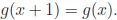
Here A and B are parameters. The meaning of taking modulus (mod 1) is to keep the fraction part of the result, throwing away its integer part. In (1.2) g(x) is a function of period 1:

The symbolic dynamics of circle maps, whose phase space is a closed circle, has some distinctive new features. Chapter 4 will be devoted to its study.

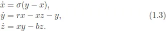
The Lorenz model

The thermal convection above a flat earth surface is described by a set of partial differential equations. After much simplification it may be reduced to a set of three ordinary differential equations (Saltzman [1962], Lorenz [1963]):

It is known as the Lorenz model. The three-dimensional phase space is spanned by the three coordinates x, y, and z. There are three parameters σ, b, and r. Usually two of the three parameters are kept constant, e.g., σ = 10, b = 8/3. Many periodic and chaotic orbits are observed when r is varied over a wide range, say, from 1 to 350. The aperiodic orbit observed by Lorenz at r = 28 was one of the earliest examples of strange attractors.

The Lorenz model (1.3) has a discrete symmetry: it remains unchanged when the signs of x and y are reversed while z is kept unchanged. In other words, it is invariant under the transformation x → −x, y → −y, and z → z. This anti-symmetry makes the Lorenz model close to the following one-dimensional anti-symmetric cubic map

and a few other 1D maps with the same symmetry.

The anti-symmetric and more general cubic maps provide a bridge to maps with many monotone branches. These important maps call for extension of the symbolic dynamics of unimodal case to maps with multiple critical points and discontinuities. This will be studied in Chapter 3.

Periodically forced systems

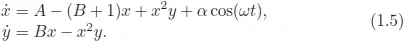
Many ordinary differential equations with two variables are nonlinear oscillators. The most complex behavior in such planar systems is periodic motion. Chaotic motion cannot appear. However, if a planar system is driven by periodic external force, chaotic behavior may come into play. There are many systems incorporating the interplay between the internal and external frequencies. For example, the periodically forced Brusselator

Another example is the forced Duffing equation, which describes the nonlinear oscillation of a magnetic bea...

Table of contents

• Cover page
• Title page
• Copyright
• Preface to the Second Edition
• Preface to the First Edition
• Contents
• 1 Introduction
• 2 Symbolic Dynamics of Unimodal Maps
• 3 Maps with Multiple Critical Points
• 4 Symbolic Dynamics of Circle Maps
• 5 Symbolic Dynamics of Two-Dimensional Maps
• 6 Application to Ordinary Differential Equations
• 7 Counting the Number of Periodic Orbits
• 8 Symbolic Dynamics and Grammatical Complexity
• 9 Symbolic Dynamics and Knot Theory
• 10 Appendix
• References
• Index