Key Concepts in Sport and Exercise Research Methods

Michael Atkinson

• Publisher: SAGE Publications Ltd
• Year: 2011
• Print ISBN: 9781848607293, 9781848607286
• eBook ISBN: 9781446292020
• Edition: 1
• Topic: Social Sciences
• Subtopic: Social Science Research & Methodology
• Index: Social Sciences

"What a helpful book! This will be a ?friend ? to many undergraduate students looking for clarification."
- Helen Hazelwood, St Mary?s University College

"This is a great book that really helps the students understand research and the complex processes that can often daunt even the most intelligent students."
- Phil Barter, Middlesex University

"Few can bring research methods to life like Mike Atkinson. His breadth of research interests and experience mean he can introduce you to all you need to know and inspire you to get down to doing some research yourself."
- Dominic Malcolm, Loughborough University

This book systematically demonstrates the significance and application of research methods in plain language. Written for students, it contains the core methodological concepts, practices and debates they need to understand and apply research methods within the field of sport and exercise. It provides a comprehensive panoramic introduction which will reassure and empower students.

Written by a leading academic and drawing on years of teaching experience, it includes carefully cross-referenced entries which critically engage with interdisciplinary themes and data. Each concept includes:

• clear definitions
• suggestions for further reading
• comprehensive examples
• practical applications

Pragmatic, lucid and concise the book will provide essential support to students in sports studies, sport development, sport and exercise science, kinesiology and health.

Descriptive Statistics

Descriptive statistics often get a bad rap in research circles. In research methods classes, they are discussed quite quickly in an introductory undergraduate course and then scarcely mentioned in subsequent courses. They are like the nerdy little brother of their more socially popular big brother, inferential statistics. Descriptive statistics are used to describe the basic features of the data in a study. They provide simple summaries about the sample and the measures. Together with simple graphics analysis, they form the basis of virtually every quantitative analysis of data. Learning the place of descriptive statistics in quantitative research is foundational, and several of the descriptives are entry points into advanced and inferential statistics.

WHAT IS THIS CONCEPT?

I consider myself to be a serious (serious, to me, that is!) recreational athlete, and I am a vegan. For several years friends and nutritionists have warned me about the risks associated with being a vegan and engaging in endurance athletics. Nutritionists have instructed me to be very mindful of striking a complete mineral balance in my daily food intake, or else I run the risk of losing bone mineral density. This is dangerous because of the punishment inflicted on the bones through long bouts of running on roads, weight training and some of the other activities accompanying my tastes for sport. For the last seven years I have been very cautious and conscientious about my eating habits, and have been able to maintain a healthy bone structure. What about other vegan (and non-vegan) endurance athletes? What do their bones look like? How could a researcher acquire a straightforward portrait of bone mineral density among a group of endurance athletes?

Here come descriptive statistics to the rescue! Because I am naturally curious, I managed to gather a group of 10 well-trained endurance athletes (5 vegan and 5 non-vegan) between the ages of 30 and 60. Each one of them agrees to visit my research lab at the university and undertake a DEXA (Dual Energy X-ray Absorptiometry) scan. A DEXA scan uses low-dose x-rays (about one tenth of the radiation dose of a chest x-ray), to assess body composition. A DEXA scan is very, very cool. While you are lying on a cushioned table, the DEXA scanner arm passes over your body taking x-rays to compile a physiological portrait of your body. The test works by measuring the density of a specific bone or bones, usually the spine, hip and wrist. The density of these bones is then compared with an average index based on age, sex and size (normally, a 30-year-old male or female). The resulting comparison is used to determine risk for fractures and the stage of osteoporosis in an individual. Bone mineral density is computed as BMC/W [g/cm²]: where BMC = bone mineral content = g/cm; and W = width of bone at the scanned line. Average density scores for a healthy 30-year-old are approximately 1,500 kg m⁻³. Now, raw scores are typically transformed into T or S scores for patient comparisons with the expected norm, but let’s not get too complicated right now.

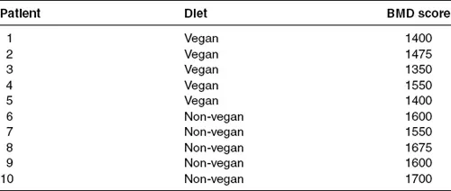
I conducted a DEXA scan on each of my 10 athletes and compiled the results in Table 1. In this table, I have presented scores on two variables I measured among the athletes: their diet and their average bone mineral density scores. Let’s focus on the second. In most research scenarios, we run a preliminary analysis of the variables, one at a time, we are centrally concerned with as a means of examining how they are ‘behaving’ in our sample. Remember the purpose of my data gathering exercise is to compare the bone mineral density of vegan athletes to their non-vegan peers. But let’s not rush too quickly into a comparison between the two groups.

Descriptive statistical analysis is predominantly univariate, focusing on one variable at a time; and we have a portfolio of descriptive statistics to examine the characteristics of each variable in our sample. Each is used to reduce a set of total scores on each variable, like bone mineral density scores, in a sensible and meaningful way. The arithmetic average or mean for a variable is one such statistic. What if we wanted to know how well a major league baseball player is performing offensively during a year? Would it make sense to examine all of his at bats for 162 games during the season? No chance! Or, would I simply look at the number of hits he made in the year to assess his offensive prowess? Probably not, because hits do not tell me anything about how many chances to hit the player received over the season. One hundred hits in 100 at bats means something entirely different than 100 hits in 673 at bats! The preferred descriptive statistic in baseball is the batting average. This single number is the player’s total hits divided by the number of times at bat. A batter who is hitting .333 is getting a hit one time in every three at bats; one batting .250 is hitting one time in four. The batting average captures and summarises performance over a large number of discrete events (at bats). Batting averages provide us with a first estimate of batter performance and variability in performance over the year.

Table 1 Diet and bone mineral density

Descriptive statistics reveal more than mere numeric averages for a variable of interest. Descriptives provide references points to highs, lows, middle-points, and the dispersion of scores around central anchors in our data. They quantify how much difference there is between people’s scores on a particular variable, and therefore provide researchers with an indicator of the distribution of scores in a sample. So just by running a set of descriptive statistics on my gathered bone mineral density scores, I could summarise average density in the group, the range of scores (highest and lowest), and the amount of difference, and even average amount of difference, between people in the group. All of these statistics are critical for understanding how bone mineral density scores are distributed among the athletes.

WHY IS THIS RELEVANT TO ME?

The relevance of descriptive statistics is manifold, but three reasons stand out. First, they are our preliminary measures of a variable’s ‘behaviour’ in our sample. Do people all score around the same on the variable? How do people score on average? How do scores cluster around the average? What is the highest and lowest people score? Just imagine if I measured bone mineral density among 9,894 athletes with a range of different diets, and they had an average of 1,576 kg m⁻³. In fact, almost all of the athletes scored exactly that BMD value. Very interesting! These preliminary data tell me that diet does not seem to affect bone mineral density scores.

Second, and related to the above, most of the advanced statistics you will encounter as a student are predicated on two simple descriptive statistics, the mean (noted in statistical terms as

and the standard deviation (noted in statistical terms as s). The mean is the arithmetic average of scores in a particular variable and the standard deviation is a measure of how far away a typical person is in the sample from the mean score (we will discuss these in a bit more detail below). The mean tells us about the average in the distribution of gathered scores, and the standard deviation how much average difference there is between people’s scores on the variable. The more people’s scores vary in a sample, the greater the standard deviation. In our sample data of bone mineral density for the 10 athletes, the mean is 1,530 kg m⁻³ and the standard deviation is ± 120.07 kg m⁻³. What does this tell us? Well, the average person in our sample scores slightly above the expected BMD score for a healthy person; and, on average, a person scores 120.07 away from the mean (that is, either above or below it). Means and standard deviations are usually reported together, such as, ‘Bone mineral density among the athletes had a mean of 1,530 kg m⁻³ [± 120.07].’ Or, we could simply write, ‘Bone mineral density in the sample of athletes was

= 1,530 kg m⁻³ [± 120.07].’

Third, we can extend the univariate basis of descriptive statistics to multivariate analysis. Through the use of crosstabs, simple bar or line graphs and frequency distribution charts, we can compare how sets of scores on two variables match up. For example, what do we learn from Table 2?

What do the data shown in Table 2 teach us about the potential relationship between diet and bone mineral density? First, it reveals that on average, vegans do seem to have lower bone mineral density scores than non-vegans. Vegans seem to score, on average, below what is expected for a typical healthy adult. This is an important finding because the mean of the sample before we separated them analytically into two sub-groups was 1,530 kg m⁻³. So it seems the non-vegans are pulling the mean up!

Table 2 Bone mineral density means and standard deviations

Diet	Mean BMD score
Vegan	1435 [± 78.25]
Non-vegan	1625 [± 61.24]

What becomes even more interesting is that the standard deviation for the vegans is higher than for non-vegans, meaning there is more variability within their group. Higher variability may indicate that diet does not affect all vegans in the same manner. All of these preliminary insights illustrate important lessons about bone mineral density in the sample.

SHOW ME HOW IT’S USED!

Everything in statistics depends on the measurement process. Everything … really, it’s true. How I have chosen to measure a variable determines what statistical analyses I may run on said variable in every case, and the process commences with descriptive statistics. Depending on whether you are confronted with a continuous variable (one measured or scored as a ‘naturally occurring’ number, like age or weight) or a discrete/categorical variable (one in which the response categories are measured by words or phrases that are turned into numbers through the coding process … like your religion, place of birth, or favourite physical activity), your descriptive statistics options then follow.

Let’s begin with discrete variables. For variables with distribution parameters set by words or phrases, there are not a million and one options for descriptive statistical analysis. When we analyse the behaviour of a discrete/categorical variable we have measured, a frequency distribution analysis is normally the point of departure. A frequency distribution lists in tabular form, or presents in graphic form (e.g. a bar chart such as a histogram, pie diagram, or other), how people have scored on the variable. Frequency analysis is rather straightforward in that it provides a visual summary and breakdown of a discrete variable’s distribution as either the number of people scoring for each category of the variable or the percentage of people in the sample scoring on that category.

Now, continuous variables are another story entirely. We could commence the statistical analysis of the distribution of a continuous variable with a frequency analysis as in the case above (i.e. through a histogram, scatterplot or line graph) but there are three other sub-sets of descriptive statistical analysis at our disposal as well. First, we might examine the ‘holy trinity’ of all descriptive statistics: the mean, median and mode. The mean we have covered already – it is the arithmetic average of scores on a particular variable. The mode is the most frequently occurring score in our sample, and the median is the score in the sample at which 50% of the sample falls below and 50% above. Together, all of these statistics are referred to as measures of central tendency. Individually and collectively they provide a snapshot of where an average or typical person in the sample scores.

The Mean, Median and Mode: An Example

We measure V0₂ max scores among a group of 11 well-trained athletes. The scores are as follows:

50, 58, 59, 59, 59, 67, 69, 70, 70, 72, 76

Mean: 64.45, because [50, 58, 59, 59, 59, 67, 69, 70, 70, 72, 76 / 11 = 64.45]

Median: 67, because five scores fall below and five above.

Mode: 59, because three people scored 59 in the sample, more than for any other score.

The second sub-set of descriptive statistics at our disposal is called measures of dispersion or spread. These statistics provide an additional layer of information about the range of the scores in the distribution, the degree of variability in scores, and the relative shape of the distribution of scores. Three commonly used measures of dispersion are worth noting. The range is the difference between the highest and lowest scores in a sample. The range for V0₂ max in the box above would be 76–50 = 26. The range tells us how ‘wide’ the distribution is in the sample. The other two measures of dispersion we report are the variance and the standard deviation. The variance is computed as the average squared deviation of each score from the mean (complex, I know), and the standard deviation, remember, is the average distance of any person in the sample from the mean. We rarely report the latter and instead focus on the former. The standard deviation is an incredibly widely used statistic for reporting the degree of variability in the sample, and it is read in conjunction with the mean. If the standard deviation gets closer to zero, we know scores hover closely around the mean. As the standard deviation inflates, we know scores are spread out more widely away from the mean. So, if the mean gives an estimate of the average VO₂ max, the standard deviation would tell us whether people all score around 64.45 or if the mean is only a central point in a se...

Table of contents

• Cover Page
• Title
• Copyright
• Contents
• List of Figures and Tables
• About the Author
• Introduction: Using this Book
• Academic Journals
• Analytic Epidemiology
• Applied vs. Pure Research
• Archival Research
• Causality
• Critical theory
• Descriptive Statistics
• Discourse Analysis
• Distributions
• Epistemology
• Ethnography
• Evaluation Research
• Evidence-Based Research and Practice
• Experiments
• Grounded theory
• Hypotheses
• Inferential Statistics
• Interdisciplinary Research
• Interpretivism
• Interviewing
• Literature Reviews
• Media Analysis
• Meta-Analysis
• Ontology
• Populations and Samples
• Positivism
• Quantitative vs. Qualitative Research
• Questionnaires
• Reliability
• Representation
• Research Ethics
• Research Proposals
• Research Questions
• Theory
• Translation
• Triangulation
• Unobtrusive Methods
• Validity
• Variables
• Visual Methods