Introducing LISREL

A Guide for the Uninitiated

Adamantios Diamantopoulos, Judy A Siguaw

• Publisher: SAGE Publications Ltd
• Year: 2000
• Print ISBN: 9780761951711, 9780761951704
• eBook ISBN: 9781446226599
• Edition: 1
• Topic: Social Sciences
• Subtopic: Social Science Research & Methodology
• Index: Social Sciences

`If you encounter a research student for whom the very word LISREL induces feelings of fear, quietly recommend that they read this book. They will thank you for it. With increasingly user-friendly versions of LISREL being released and guide books such as this published, LISREL really should be accessible to all? - European Journal of Marketing

Emphasizing substantive issues rather than intricate statistical details, this book provides a comprehensive introduction to LISREL for structural equation modeling (SEM) using a non-technical, user-oriented approach that. The emphasis is on:

- exposing the reader to the major steps associated with the formulation and testing of a model under the LISREL framework

- describing the key decisions associated with each step

- highlighting potential problems and limitations associated with LISREL modeling

- assisting the interpretation of LISREL input and output files.

The overall aim is to provide a critical understanding of what is really involved in LISREL modeling and sensitize the reader against `mechanically? fitting or modifying models.

The entire range of decisions associated with the practical application of the LISREL program is covered in a user-friendly fashion. Concrete examples are used throughout to illustrate issues relating to model conceptualization, specification, identification, estimation, evaluation, modification, and cross-validation and illustrated with actual program output.

The program is made much more accessible by adopting the more user-friendly SIMPLIS command language for preparing input files. Although primarily aimed at beginning users, readers are directed to further reading together with a comprehensive bibliography for the more advanced user.

---

1 WHAT IS LISREL ALL ABOUT?

---

‘Man’s the only species neurotic enough to need a purpose in life’

David Nobbs, The Fall and Rise of Reginald Perrin

An acquaintance of yours has been trying for some time to set you up with a blind date. Since you have hit a dry spell in the dating scene lately, you begin giving the set-up more serious consideration. From your discreet enquiries, you have been able to determine that the potential date has a ‘great personality’. Having experienced particularly bad blind dates in the past during which you were either terminally bored by the date’s incessant chatter or frightened to death by your date’s appearance, you feel almost certain that this great personality relegates this person into the ‘dog’ classification in terms of sex appeal! However, being the great researcher you are, you decide to test the relationship between sex appeal and personality to see if your belief that unappealing physical looks equate to a great personality is actually justified.

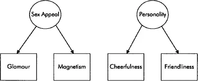
So, you have two constructs you must measure — personality and sex appeal. You obviously need to collect data on these constructs to test your hypothesized relationship, but neither construct is easily observed; both are latent variables. So how can they be measured? You could, for example, subjectively rate (e.g. on a scale from 1 to 10) various aspects of personality and sex appeal that can be observed. For example, personality might be measured by ‘cheerfulness’ or ‘friendliness’; similarly, sex appeal might be measured by ‘glamour’ or ‘magnetism’. These measurable indicators of personality and sex appeal are known as manifest variables. Figure 1.1 illustrates the relationships between the latent variables and their indicators.¹ Note that, according to the direction of the arrows, each manifest variable is depicted as being determined by its underlying latent variable (as in factor analysis). In other words, manifest variables reflect latent variables; for this reason they are known as reflective indicators (this is an important point, to which we shall return in later chapters).

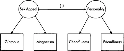
According to your ‘theory’, sex appeal is a determinant of personality (because very good-looking people don’t have to develop as pleasing personalities as average-looking individuals to attract members of their own and/or opposite sex). So, in your study, sex appeal would be the independent variable because it acts as a determinant of personality. Personality, on the other hand, would be the dependent variable because it is influenced by, or is an effect of sex appeal. Now, if a variable is not influenced by any other variable in the model, the variable is an exogenous variable; exogenous variables act always as independent variables. Variables which are influenced by other variables in the model are known as endogenous variables. In our example, sex appeal would be an exogenous and personality an endogenous variable. Note that endogenous variables can affect other endogenous variables, i.e. they can act as both independent and dependent variables. Figure 1.2 shows the relationship between the latent variables in the model, the sign of the arrow indicating the expected direction of the link. Conceptually, the model of Figure 1.2 is very similar to a simple regression model with one predictor (i.e. independent) and one criterion (i.e. dependent) variable. The key difference is that, in the present case, the variables involved are latent, each measured by multiple indicators. As you might have guessed, conventional regression techniques cannot be used to estimate models such as the one depicted in Figure 1.2. It is here where LISREL and other similar methodologies – which are designed to deal with latent variables – come in handy; however, before we start telling you about LISREL, we need to briefly mention one very important concept, namely error.

Figure 1.1 Latent and manifest variables

Figure 1.2 A relationship between two latent variables

In both Figure 1.1 and 1.2, we ‘conveniently’ assumed away any imperfections in our measurements and/or predictions. In Figure 1.1 we (implicitly) assumed that our manifest variables are perfect measures of the two latent constructs, i.e. that there is no measurement error present. However, this is a rather unrealistic assumption as it is highly unlikely that empirical measurements will exhibit perfect validity or reliability; thus we should make allowances for the fact that we are dealing with fallible measures, i.e. imperfect representations of latent variables (particularly when subjective ratings are used, as is the case with most measures in social science research). Similarly, in Figure 1.2, there is the rather heroic assumption that personality is solely and fully determined by sex appeal, which is as realistic as saying that ‘it never rains in England’. To the extent that other variables (not included in the model) have an influence on personality, then there will be unexplained variation of the latter; thus we need to include a residual term (or ‘disturbance’) in order to account for those influences on personality that have not been explicitly modeled.

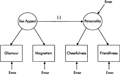
Figure 1.3 Incorporating error

Figure 1.3 shows a modified version of Figure 1.2, incorporating both measurement error (also known as ‘error in variables’) and structural error (also known as ‘error in equations’). LISREL allows you to examine the relationships between latent variables (so you can test your substantive theory) as well as the relationships between the latent variables and their indicators (so that you can judge the quality of your measures). In fact, fitting a LISREL model to Figure 1.3 would tell you whether sex appeal has a negative effect on personality (as opposed to a positive or no effect); how strong that effect is (i.e. how much of the variation in personality can be ‘explained’ by sex appeal); and how good your measures of sex appeal and personality are (i.e. how well they are capturing the latent variables). Obviously, in order to fit a LISREL model to Figure 1.3 you need (a) some data, and (b) some knowledge on how to use LISREL. While we cannot help you with the former task (i.e. data collection), we hope to be of assistance with the latter.

A brief background

The term LISREL is an acronym for LInear Structural RELationships and, technically, LISREL is a computer program which was developed by Karl G. Jöreskog and Dag Sörbom to do covariance structure analysis² (see Appendix 1A for a brief explanation of variance and covariance). However, the program has become so closely associated with covariance structure models that such models are often referred to as LISREL models. Covariance structure models are widely used in a number of disciplines, including economics, marketing, psychology and sociology. They have been applied in investigations based on both survey and experimental data and have been used with cross-sectional as well as longitudinal research designs.³

Although the LISREL model remains basically the same today as when it first appeared in the early 1970s, subsequent revisions of the computer program have incorporated developments in statistical and programming technology to arrive at the current LISREL 8 version, which is the version used in this book.⁴ In recent years, other software packages⁵ have attempted to usurp LISREL’s commanding position as the preferred software for covariance structure analysis, but LISREL has managed to defend its corner. Hence, this book focuses on doing covariance structure analysis utilizing the LISREL program; however, having mastered the principles of undertaking covariance structure analysis with LISREL, you should be able to adapt your knowledge and find little difficulty in using other similar programs.

Covariance structure analysis is a multivariate statistical technique which combines (confirmatory) factor analysis and econometric modeling for the purpose of analyzing hypothesized relationships among latent (i.e. unobserved or theoretical) variables measured by manifest (i.e. observed or empirical) indicators. A full covariance structure model is typically composed of two parts (or sub-models). The measurement model describes how each latent variable is measured or operationalized by corresponding manifest indicators; for example, we previously suggested that glamour and magnetism might be manifest indicators of the latent variable, sex appeal. The measurement model also provides information regarding the validities and reliabilities of the observed indicators. The structural model, on the other hand, describes the relationships between the latent variables themselves and indicates the amount of unexplained variance. Using our earlier example, then, the structural model would explain whether there is a significant negative relationship between sex appeal and personality, and would also indicate to what degree personality is determined by factors other than sex appeal.⁶

Covariance structure analysis is confirmatory in nature in that it seeks to confirm that the relationships you have hypothesized among the latent variables and between the latent variables and the manifest indicators are indeed consistent with the empirical data at hand. Confirmation (or lack of) is accomplished by comparing the computed covariance matrix implied by the hypothesized model to the actual covariance matrix derived from the empirical data (see Appendix 1B for an explanation of the ‘implied covariance matrix’). Because this type of analysis utilizes the covariance matrix rather than the individual observations as input, covariance structure modeling is an aggregate methodolo...

Table of contents

• Cover Page
• Title
• Copyright
• Dedication
• Contents
• About the authors
• Preface
• Acknowledgements
• 1 What is Lisrel All About?
• 2 Model Conceptualization
• 3 Path Diagram Construction
• 4 Model Specification
• 5 Model Identification
• 6 Parameter Estimation
• 7 Assessment of Model Fit
• 8 Model Modification
• 9 Model Cross-Validation
• 10 An Introduction To Prelis 2
• References
• Index