Elegant Fractals

Automated Generation of Computer Art

Julien Clinton Sprott

• Publisher: WSPC
• Year: 2018
• ISBN:
  9789813237155
• Topic: Computer Science
• Subtopic: Data Modelling & Design
• Index: Computer Science

Fractals are intricate geometrical forms that contain miniature copies of themselves on ever smaller scales. This colorful book describes methods for producing an endless variety of fractal art using a computer program that searches through millions of equations looking for those few that can produce images having aesthetic appeal. Over a hundred examples of such images are included with a link to the software that produced these images, and can also produce many more similar fractals. The underlying mathematics of the process is also explained in detail.

Other books by the author that could be of interest to the reader are Elegant Chaos: Algebraically Simple Chaotic Flows (J C Sprott, 2010) and Elegant Circuits: Simple Chaotic Oscillators (J C Sprott and W J Thio, 2020).

Contents:

• Preliminaries
• Search Techniques
• Iterated Maps
• Chaotic Flows
• Iterated Function Systems
• Escape-time Plots
• Spatiotemporal Systems
• Random Fractals
• Fractal Tessellations
• Epilog

Readership: Student, professional and general public.
Key Features:

• VISUAL ELEGANCE - It provides an automated method for producing interesting fractals with over a hundred full-color examples
• ACCESSIBLE COMPUTATION - It describes the mathematics behind the creation of fractals
• "DO-IT YOURSELF TOO!" TECHNOLOGY ENGINE - It provides a link to software behind the generation of countless additional examples

Chapter 1

Preliminaries

This chapter will introduce some of the fractal and chaos concepts and terminology so that the book is self-contained and readable even if you are unfamiliar with the subject. It will also describe how the images are produced using the Hénon map as the main example. It should enable you to get a quick start producing your own elegant fractal images.

1.1Fractals

Fractals have existed since the beginning of time and are all around us, but only in the last few decades have they been widely recognized and properly described. A fractal is a geometric object that contains miniature copies of itself and is thus said to be self-similar. In fact, a true mathematical fractal contains infinitely many copies of itself on ever smaller scales. Mathematical fractals, just like mathematical points and lines, have never been seen and exist only in the minds of mathematicians. When you draw a point or a line, you give it a small width to make it visible, and in so doing it is no longer a true point or line. So it is with the fractal objects in nature and the images that constitute the subject of this book.

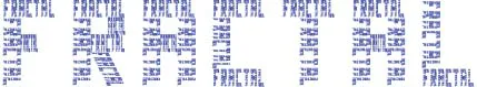
A whimsical example of the kind of fractal we will be considering is the word ‘FRACTAL’ in Fig. 1.1, which is only visible because the process of miniaturization is stopped before the infinitely many points that make up the image become too small to see. Technically, it is called a prefractal, and all fractals in nature are of this sort. Even worse, most natural fractals are self-similar only in a rough statistical sense. You will never find exact copies of the whole upon magnifying a portion of them. Clouds, mountains, and rivers are common examples of fractals in nature.

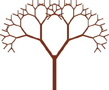
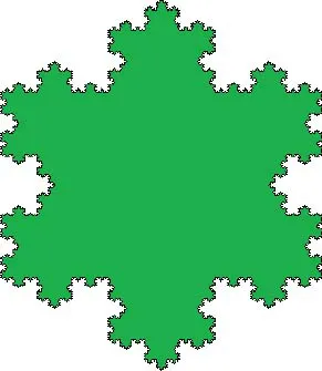
Other examples of natural objects that are usually called fractals are trees and coastlines, shown in stylistic form in Figs. 1.2 and 1.3, respectively. In a tree, the branches have branches which have branches, ad infinitum. A coastline or a river has bends that have smaller bends, ad infinitum. A coastline is not a line at all, and any attempt to measure its length will frustrate you because the result will depend on the length of the ruler you use to measure it, and your estimate of the length will grow ever larger without limit as you improve your measurement. The object in Fig. 1.3 is called a Koch snowflake or Koch island, named after the Swedish mathematician Helge von Koch (1904), and we will return to it toward the end of Chapter 9.

Fig. 1.1A self-similar geometric object (a fractal).

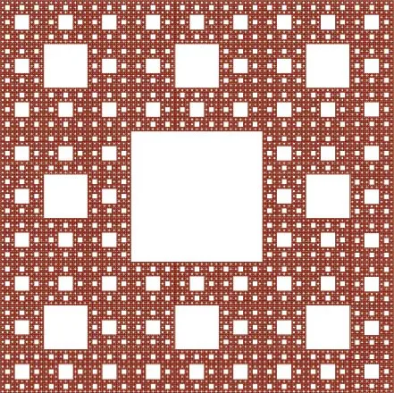
Another classic example of a mathematical fractal is the Sierpiński carpet (or Sierpiński gasket) shown in Fig. 1.4, which was first described by the Polish mathematician Wacław Sierpiński (1916). It is not a very good carpet to cover your floor because it has infinitely many holes of arbitrarily small size. In fact, there is a sense to be described shortly in which it is all holes. Every point on the carpet is arbitrarily close to a hole, and the carpet itself has zero area. If you were to have such a carpet made for your bedroom, the material cost should be zero, but the labor cost would be infinite!

The previous examples of fractals are embedded in the two-dimensional plane. Fractals can also be embedded in higher dimensions. Indeed, a fractal tree usually lives in three-dimensional space, and so the image in Fig. 1.2 might better be considered as the shadow of a tree on the ground.

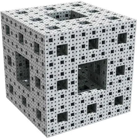
The Menger sponge [Menger (1928)] in Fig. 1.5 is an example similar to the Sierpiński carpet but embedded in three-dimensions. In fact, each face of the sponge is a Sierpiński carpet. The Menger sponge has infinite surface area but zero volume. Fractals can also be embedded in dimensions higher than three, and we will soon discuss ways to display and visualize them.

Objects such as these were proposed and studied over a hundred years ago, but even most mathematicians considered them to be monstrosities of no practical interest. Only in the 1980s did Mandelbrot (1982) bring them to the attention of a wide audience and demonstrate their relevance to patterns and processes that are ubiquitous in nature.

Fig. 1.2A stylized fractal tree.

Fig. 1.3A stylized fractal coastline.

Fig. 1.4Sierpiński carpet (a classic fractal object).

1.2Two-dimensional Maps

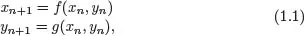
Whatever images you produce will presumably need to be displayed on a two-dimensional computer screen or piece of paper, although 3-D printers raise additional interesting possibilities. Thus it is reasonable to begin by considering a two-dimensional iterated map,

where x will be taken as the horizontal position of a point in the image and y will be taken as the vertical position of that point. Beginning with some initial condition (x₀, y₀), the equations are repeatedly solved (iterated) to determine the position of successive points (x_n, y_n) in a kind of mathematical feedback operation. The functions f and g determine the shape of the resulting object after plotting the points for several million such iterations. Interesting patterns are produced only when at least one of the functions is nonlinear, and even then, it is far from guaranteed.

Fig. 1.5Menger sponge (a classic fractal object embedded in three dimensions).

If f and g are linear functions of the form f, g = ax_n + by_n + c, successive iterates will either approach a point in the plane (a stable fixed point) or will wander off to infinity, neither of which will produce a fractal pattern. The nonlinearity is necessary to allow x and y to grow but to make the orbit fold back on itself rather than going to infinity. We say that such an orbit is bounded.

1.3The Hénon Map

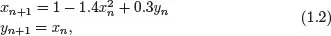
Consider the famous example of the Hénon map [Hénon (1976)] in which f(x, y) = 1 – 1.4x² + 0.3y and g(x, y) = x giving

which can be written in a more compact form as

Systems that can be written in such a form are called scalar time-delay maps since they involve a single scalar variable x and its values at some number of previous times. A scalar is a quantity that is described by a single number as opposed to a vector that requires more than one such number. For example, temperature is a scalar, but wind velocity is a vector since it has both a magnitude and direction.

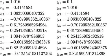
In the Hénon map, the single nonlinearity is in the x² term, and thus it is the algebraically simplest two-dimensional map whose iterates produce a fractal pattern, a so-called quadratic map. For most of the examples in this book, any small values will suffice as initial conditions, and unless otherwise noted, they will be taken as 0.1 since zero will often be an equilibrium point from which the orbit cannot escape, although that is not the case for the Hénon map. For Eq. (1.2) with x₀ = 0.1 and y₀ = 0.1, the next few iterates are given by

The iterates continue to fluctuate between the limiting values of x_min = –1.2846638 and x_max = 1.27297362 without ever repeating for as long as you care to iterate. Note that y is just the previous value of x, and so they have the same limiting values (y_min = x_min and y_max = x_max). It is useful to determine the limiting values (x_min and x_max) before plottin...