In this final chapter, we will look at expanding QGIS. We will look at combining tools into a model using the model builder. This effectively allows us to build our own reusable model, using parameters we either hardcode in or leave to the user to adjust. We will look at the ever-increasing range of plugins, before finally taking a brief look at the Python command line, where we can create scripts in the future as confidence grows with QGIS.
You may recall that in the Chapter 6, Spatial Processing we ran several tools to utilize the zonal histogram answer to the distribution of terrains (Landcover) in a buffered pipeline corridor. Open a new QGIS project and load in the Pipeline layer and the Landcover.
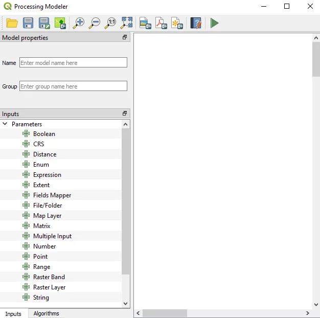
To create a model, go to Processing | Graphical Modeler to open the modeler, where we can select from different Inputs and Algorithms for our model. Graphical Modeler is shown in the following screenshot:
The Graphical Modeler
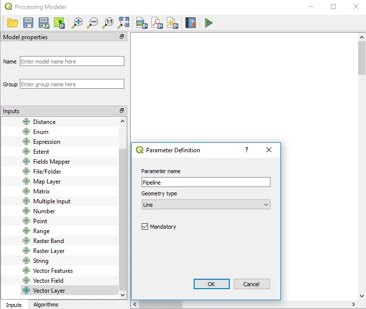
Select the Inputs tab and choose Vector Layer. Add a new parameter called Pipeline and set Geometry type to Line; this is shown in the following screenshot:
Creating a Pipeline attribute as a Geometry type—Line
Click on OK. Now, add Raster Layer and call it Landcover. In the Algorithms tab, we can use the filter at the top to narrow down our search for the correct algorithm. Search for buffer and double-click to open the algorithm. Fill in Distance as 15000 and check the box to make sure the layer is dissolved.
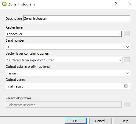
Now, search for and open the Zonal histogram tool and change the prefix to Terrain_. This is our final output so tell the model it is the final result. The final output is what is returned to the user once the model has been successfully run. The inputs should look like the following dialog box:
Zonal histogram tool
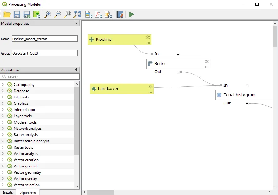
Click on OK. To finish the model, we need to enter a model Name (Pipeline_impact_terrain) and a Group name (QuickStart_QGIS). Processing will use the Group name to organize all the models that we create into different toolbox groups. The model is now complete. The finished model will look like this:
The Graphical Modeler with the model displayed
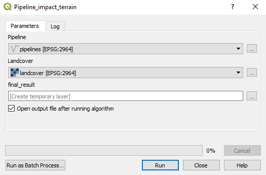
Click the save icon and save as terrain_stats.model3. Click on the green triangle or press F5 to run the model. A dialog box should appear as follows:
The model represented as a tool
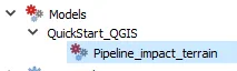
Click on Run to execute the model. The pipeline output will appear in the QGIS map window. After closing the modeler, we can run the saved models from the toolbox like any other tool. Look in Processing Toolbox under Models. This newly created model will appear there, as shown in the following screenshot. It is even possible to use one model as a building block for another model:
Model appears in the Processing Toolbox under Models
Another useful feature is that we can specify a layer style that needs to be automatically applied to the processing results. This default style can be set by right-clicking and selecting Edit, rendering styles for outputs in the context menu of the created model in the toolbox. This means that you can automate building maps if you wish.
You can share your models by giving the .model3 file to others. This is the first step in expanding the use of QGIS. Save your project.
![]()
We briefly touched on plugins in Chapter 5, Creating Maps. We used qgis2web to convert our Alaska map into a web map. The top plugins by download are listed here: https://plugins.qgis.org/plugins/popular/. You can use this page to search for plugins or look at tags to view the different plugins and their capabilities.
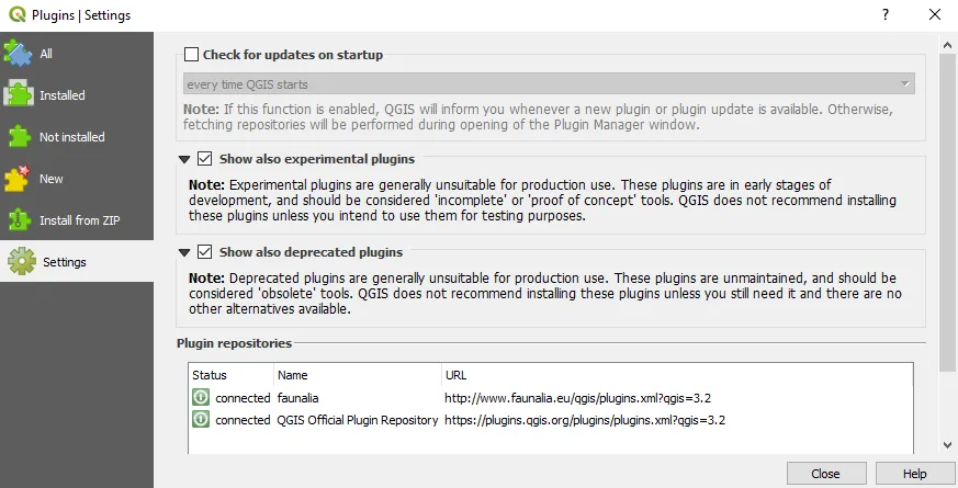
Plugins are accessed via the Plugins menu. Some plugins are experimental. By experimental, we mean they could be unstable or in the early stages of development, but it is worth turning these on in case a plugin is available that might help your workflows; just use them with caution. From the Plugins dialog, choose Settings and check the box next to Show also experimental plugins:
Plugin settings
![]()
The Semi-Automatic Classification Plugin (SCP) for QGIS allows for the supervised classification of remote sensing images, providin...