The array type in Julia is parameterized by the type of its elements and the number of its dimensions. Hence, the type of an array is represented as Array{T, N}, where T is the type of its elements, and N is the number of dimensions. So, for example, Array{UTF8String, 1} is a one-dimensional array of strings, while Array{Float64,2} is a two-dimensional array of floating point numbers.
Type parameters
You must have realized that type parameters in Julia do not always have to be other types; they can be symbols, or instances of any bitstype. This makes Julia's type system enormously powerful. It allows the type system to represent complex relationships and enables many operations to be moved to compile (or dispatch) time, rather than at runtime.
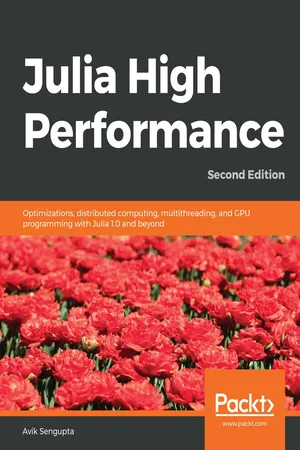
Representing the type of its element within the type of arrays as a type parameter allows powerful optimization. It allows arrays of primitive types (and many immutable types) to be stored inline. In other words, the elements of the array are stored within the array's own primary memory allocation.
In the following diagram, we illustrate this storage mechanism. The numbers in the top row represent array indexes, while the numbers in the boxes are the integer elements stored within the array. The number in the bottom row represent the memory addresses where each of these elements are stored:
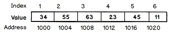
In most other dynamic languages, all the arrays are stored using pointers to their values. This is usually because the language runtime does not have enough information about the types of values to be stored in an array, and hence, cannot allocate the correctly sized storage.
As represented in the following diagram, when an array is allocated, the contiguous storage simply consists of pointers to the actual elements, even when these elements are primitive types that can be stored natively in memory:
This method of storing arrays inline without pointer indirection as much as possible has many advantages and, as we discussed earlier, is responsible for many of Julia's performance claims. In other dynamic languages, the type of every element of the array is uncertain and the compiler has to insert type checks on each access. This can quickly add up and become a major performance drain.
Further, even when every element of the array is of the same type, we pay the cost of memory load for every array element if they are stored as pointers. Given the relative costs of a CPU operation versus a memory load on a modern processor, not doing this is a huge benefit.
There are other benefits too. When the compiler and CPU notice operations on a contiguous block of memory, CPU pipelining and caching are much more efficient. Some CPU optimizations, such as Single Instruction Multiple Data (SIMD), are also unavailable when using indirect array loads.
![]()
When an array has only one dimension, its elements can be stored one after the other in a contiguous block of memory. As we observed in the previous section, operating on this array sequentially from its starting index to its end can be very fast, making it amenable to many compiler and CPU optimizations.
Two-dimensional (or greater) arrays can, however, be stored in two different ways. We can store them row-wise or column wise. In other words, we can store from the beginning of the array the elements of the first row, followed by the elements of the second row, and so on. Alternatively, we can store the elements of the first column, then the elements of the second column, and so on.
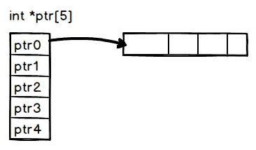
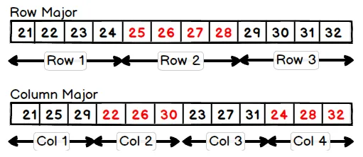
Consider, in the following diagram, the matrix with three rows and four columns:
This matrix can be stored in two different ways, as illustrated in the following diagram. In the Row Major option, the elements of a row are stored together. In the Column Major option, the elements of a column are stored together:
Arrays in C are stored as row-ordered. Julia, on the other hand, chooses the latter strategy, storing arrays as column-ordered, similar to MATLAB and Fortran. This rule generalizes to the higher-dimensional array as well; it is always the last dimension that is stored first.
Naming conventions
Conventionally, the term row refers to the first dimension of a two-dimensional array, and column refers to the second dimension. As an example, for a two-dimensional array of x::Array{Float64, 2} floats, the expression x[2,4] refers to the elements in the second row and fourth column.
This particular strategy of storing arrays has implications for how we navigate them. The most efficient way to read an array is in the same order in which it is laid out in memory. That is, each sequential read should access contiguous areas in memory.
We can demonstrate the performance impact of reading arrays in sequence with the following code that squares and sums the elements of a two-dimensional floating point array, writing the result at each step back to the same position. The following code exercises both the read and write operations for the array:
function col_iter(x)
 s=zero(eltype(x))
 for i in 1:size(x, 2)
 for j in 1:size(x, 1)
 s = s + x[j, i] ^ 2
 x[j, i] = s
 end
 end
end

function row_iter(x)
 s=zero(eltype(x))
 for i in 1:size(x, 1)
 for j in 1:size(x, 2)
 s = s + x[i, j] ^ 2
 x[i, j] = s
 end
 end
end
The row_iter function operates on the array in the first row, while the col_iter function operates on the array in the first column. We expect, based on the description of the previous array storage, that the col_iter function would be considerably faster than the row_iter function. Running the benchmarks, this is indeed what we see, as follows:
julia> a = rand(1000, 1000);


julia> @btime col_iter($a)
 1.116 ms (0 allocations: 0 bytes)

julia> @btime row_iter($a)
 3.429 ms (0 allocations: 0 bytes)
The difference between the two is quite significant. The column major access is more than twice as fast. This kind of difference in the inner loop of an algorithm can make a very noticeable difference in the overall runtime of a program. It is, therefore, crucial to consider the order in which multidimensional arrays are processed when writing performance-sensitive code.
![]()
Sometimes, you may have an algorithm that is naturally expressed as row-first. Converting the algorithm to column-first iteration can be a difficult process, prone to errors. In such cases, Julia provides an Adjoint type that can store a transpose of a matrix as a view into the original matrix. Row-wise iteration will be the fast option. We illustrate this in the following code.
julia> b=a'
1000×1000 LinearAlgebra.Adjoint{Float64,Array{Float64,2}}:
...

julia> @btime col_iter($b)
 3.521 ms (0 allocations: 0 bytes)

julia> @btime row_iter($b)
 1.160 ms (0 allocations: 0 bytes)
We see here that the timings of the function have been inverted from those in the previous section. Column iteration is now slower than row iteration. You will also notice that the time for row iteration is now the same as the column iteration was previously. This implies that using an Adjoint has no performance overhead at all.
![]()
Creating a new array is a two-step process. In step one, memory for the array needs to be allocated. The size of the memory is a product of the length of the array and the size of each element of the array (ignoring the small overhead of the type tag at the top). Second, the allocated memory n...