MrExcel 2021: Unmasking Excel delivers practical, real-world solutions for mastering Excel's most powerful features, including pivot tables, formulas, data models, and Power Query. Discover the latest enhancements, such as LET and LAMBDA functions, dynamic array formulas, and new data types, to transform your spreadsheets and gain a competitive edge. Whether you're a seasoned professional or an aspiring data analyst, this guide will empower you to become an Excel guru and unlock new levels of productivity.
- 218 pages
- English
- ePUB (mobile friendly)
- Available on iOS & Android
eBook - ePub
About this book
Unlock the full potential of Microsoft Excel with expert tips and techniques. This comprehensive guide, updated for 2021, is designed for Excel users who want to take their skills to the next level. Learn how to streamline your workflow, automate tasks, and solve complex data problems with ease.
Trusted by 375,005 students
Access to over 1.5 million titles for a fair monthly price.
Study more efficiently using our study tools.
Information
#1 Double-Click the Fill Handle to Copy a Formula
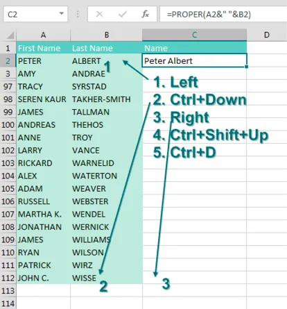
You have thousands of rows of data. You’ve added a new formula in the top row of your data set, something like =PROPER(A2&" "&B2), as shown here. You need to copy the formula down to all of the rows of your data set.

Many people will grab the Fill Handle and start to drag down. But as you drag down, Excel starts going faster and faster. There is a 200-microsecond pause at the last row of data. 200 microseconds is long enough for you to notice the pause but not long enough for you to react and let go of the mouse button. Before you know it, you’ve dragged the Fill Handle way too far.

The solution is to double-click the Fill Handle! Go to exactly the same spot where you start to drag the Fill Handle. The mouse pointer changes to a black plus sign. Double-click. Excel looks at the surrounding data, finds the last row with data today, and copies the formula down to the last row of the data set.

In the past, empty cells in the column to the left would cause the “double-click the Fill Handle” trick to stop working just before the empty cell. But as you can see below, names like Madonna, Cher, or Pele will not cause problems. Provided that there is at least a diagonal path (for example, via B76-A77-B78), Excel will find the true bottom of the data set.

In my live Power Excel seminars, this trick always elicits a gasp from half the people in the room. It is my number-one time-saving trick.
Alternatives to Double-Clicking the Fill Handle
This trick is an awesome trick if all you've done to this point is drag the Fill Handle to the bottom of the data set. But there are even faster ways to solve this problem:
- Use Tables. If you select one cell in A1:B112 and press Ctrl+T, Excel formats the range as a table. Once you have a table, simply enter the formula in C2. When you press Enter, it is copied to the bottom.
- Use a complex but effective keyboard shortcut. This shortcut requires the adjacent column to have no empty cells. While it seems complicated to explain, the people who tell me about this shortcut can do the entire thing in the blink of an eye.
Here are the steps:
1. From your newly entered formula in C2, press the Left Arrow key to move to cell B2.
2. Press Ctrl+Down Arrow to move to the last row with data—in this case, B112.
3. Press the Right Arrow key to return to the bottom of the mostly empty column C.
4. From cell C112, press Ctrl+Shift+Up Arrow. This selects all of the blank cells next to your data, plus the formula in C2.
5. Press Ctrl+D to fill the formula in C2 to all of the blanks in the selection. Ctrl+D is fill Down.
Note: Ctrl+R fills right, which might be useful in other situations.
As an alternative, you can get the same results by pressing Ctrl+C before step 1 and replacing step 5 with pressing Ctrl+V.
Thanks to the following people who suggested this tip: D. Carmichael, Shelley Fishel, Dawn Gilbert, @Knutsford_admi, Francis Logan, Michael Ortenberg, Jon Paterson, Mike Sullivan and Greg Lambert Lane suggested Ctrl+D. Bill Hazlett, author of Excel for the Math Classroom, pointed out Ctrl+R.
#2 Break Apart Data
You have just seen how to join data, but people often ask about the opposite problem: how to parse data that is all in a single column. Say you wanted to sort the data in the figure below by zip code:

Select the data in A2:A99 and choose Data, Text to Columns. Because some city names, such as Sioux Falls, are two words, you ...
Table of contents
- Dedication
- About the Author
- About the Contributors
- Foreword
- #1 Double-Click the Fill Handle to Copy a Formula
- #2 Break Apart Data
- #3 Filter by Selection
- #4 Bonus Tip: Total the Visible Rows
- #5 The Fill Handle Does Know 1, 2, 3…
- #6 Fast Worksheet Copy
- #7 Use Default Settings for All Future Workbooks
- #8 Recover Unsaved Workbooks
- #9 Simultaneously Edit the Same Workbook in Office 365
- #10 New Threaded Comments Allow Conversations
- #11 Create Perfect One-Click Charts
- #12 Paste New Data on a Chart
- #13 Create Interactive Charts
- #14 Show Two Different Orders of Magnitude on a Chart
- #15 Create Waterfall Charts
- #16 Create Funnel Charts in Office 365
- #17 Create Filled Map Charts in Office 365
- #18 Create a Bell Curve
- #19 Plotting Employees on a Bell Curve
- #20 Add Meaning to Reports Using Data Visualizations
- #21 Sort East, Central, and West Using a Custom List
- #22 Sort Left to Right
- #23 Sort Subtotals
- #24 Sort and Filter by Color or Icon
- #25 Consolidate Quarterly Worksheets
- #26 Get Ideas from Artificial Intelligence
- #27 Create Your First Pivot Table
- #28 Create a Year-over-Year Report in a Pivot Table
- #29 Change the Calculation in a Pivot Table
- #30 Find the True Top Five in a Pivot Table
- #31 Specify Defaults for All Future Pivot Tables
- #32 Make Pivot Tables Expandable Using Ctrl+T
- #33 Replicate a Pivot Table for Each Rep
- #34 Use a Pivot Table to Compare Lists
- #35 Build Dashboards with Sparklines and Slicers
- #36 See Why GETPIVOTDATA Might Not Be Entirely Evil
- #37 Eliminate VLOOKUP with the Data Model
- #38 Compare Budget Versus Actual via Power Pivot
- #39 Slicers for Pivot Tables From Two Data Sets
- #40 Use F4 for Absolute Reference or Repeating Commands
- #41 Quickly Convert Formulas to Values
- #42 See All Formulas at Once
- #43 Audit a Worksheet With Spreadsheet Inquire
- #44 Discover New Functions by Using fx
- #45 Use Function Arguments for Nested Functions
- #46 Calculate Nonstandard Work Weeks
- #47 Turn Data Sideways with a Formula
- #48 Handle Multiple Conditions in IF
- #49 Troubleshoot VLOOKUP
- #50 Use a Wildcard in VLOOKUP
- #51 Replace Columns of VLOOKUP with a Single MATCH
- #52 Use the Fuzzy Lookup Tool from Microsoft Labs
- #53 Lookup to the Left with INDEX/MATCH
- #54 Preview What Remove Duplicates Will Remove
- #55 Replace Nested IFs with a Lookup Table
- #56 Suppress Errors with IFERROR
- #57 Handle Plural Conditions with SUMIFS
- #58 Geography & Stock Data Types in Excel
- #59 Dynamic Arrays Can Spill
- #60 Sorting with a Formula
- #61 Filter with a Formula
- #62 Formula for Unique or Distinct
- #63 Other Functions Can Now Accept Arrays as Arguments
- #64 One Hit Wonders with UNIQUE
- #65 SEQUENCE inside of other Functions such as IPMT
- #66 Replace a Pivot Table with 3 Dynamic Arrays
- #67 Dependent Validation using Dynamic Arrays
- #68 Complex Validation Using a Formula
- #69 Use A2:INDEX() as a Non-Volatile OFFSET
- #70 Subscribe to Office 365 for Monthly Features
- #72 Less CSV Nagging and Better AutoComplete
- #73 Speed Up VLOOKUP
- #74 Protect All Formula Cells
- #75 Back into an Answer by Using Goal Seek
- #76 Do 60 What-If Analyses with a Sensitivity Analysis
- #77 Find Optimal Solutions with Solver
- #78 Improve Your Macro Recording
- #79 Clean Data with Power Query
- #80 Render Excel Data on an iPad Dashboard Using Power BI
- #81 Build a Pivot Table on a Map Using 3D Maps
- #82 The Forecast Sheet Can Handle Some Seasonality
- #83 Perform Sentiment Analysis in Excel
- #84 Fill in a Flash
- #85 Format as a Façade
- #86 Word Cloud using Custom Visuals in Excel
- #87 Surveys & Forms in Excel
- #88 Use the Windows Magnifier
- #90 Avoid Whiplash with Speak Cells
- #91 Customize the Quick Access Toolbar
- #92 Create Your Own QAT Routines Using VBA Macros
- #93 Favorite Keyboard Shortcuts
- #94 Ctrl+Click to Unselect Cells
- #95 More Excel Tips
- Appendix: Excel Stories
- Index
Frequently asked questions
Yes, you can cancel anytime from the Subscription tab in your account settings on the Perlego website. Your subscription will stay active until the end of your current billing period. Learn how to cancel your subscription
No, books cannot be downloaded as external files, such as PDFs, for use outside of Perlego. However, you can download books within the Perlego app for offline reading on mobile or tablet. Learn how to download books offline
Perlego offers two plans: Essential and Complete
- Essential is ideal for learners and professionals who enjoy exploring a wide range of subjects. Access the Essential Library with 800,000+ trusted titles and best-sellers across business, personal growth, and the humanities. Includes unlimited reading time and Standard Read Aloud voice.
- Complete: Perfect for advanced learners and researchers needing full, unrestricted access. Unlock 1.5M+ books across hundreds of subjects, including academic and specialized titles. The Complete Plan also includes advanced features like Premium Read Aloud and Research Assistant.
We are an online textbook subscription service, where you can get access to an entire online library for less than the price of a single book per month. With over 1.5 million books across 990+ topics, we’ve got you covered! Learn about our mission
Look out for the read-aloud symbol on your next book to see if you can listen to it. The read-aloud tool reads text aloud for you, highlighting the text as it is being read. You can pause it, speed it up and slow it down. Learn more about Read Aloud
Yes! You can use the Perlego app on both iOS and Android devices to read anytime, anywhere — even offline. Perfect for commutes or when you’re on the go.
Please note we cannot support devices running on iOS 13 and Android 7 or earlier. Learn more about using the app
Please note we cannot support devices running on iOS 13 and Android 7 or earlier. Learn more about using the app
Yes, you can access MrExcel LX The Holy Grail of Excel Tips by Bill Jelen in PDF and/or ePUB format, as well as other popular books in Computer Science & Desktop Applications. We have over 1.5 million books available in our catalogue for you to explore.